HP 15C: Weibull Distribution Calculations

HP 15C:  Weibull Distribution Calculations

Introduction

The Weibull probability density distribution function is:

f(x) = (b / Θ) * (x / Θ)^(b-1) * exp(-(x / Θ)^b)

with the lower tail cumulative distribution of (-∞ to x):

Area = 1 - exp(-(x / Θ)^b)

The area function tells us what is the probability a device lasts no more than x time units.  

Area = 1 - Survival

The survival function is the probability a device lasts more than x time units.

Survival = exp(-(x / Θ)^b)

Generally, the higher Θ is, the flatter the Weibull Distribution curve.  

What follows are four calculations regarding the Weibull Distribution.  In the following programs, store the following values first prior to running the programs:

R0 = x

R1 = b

R2 = Θ

Use whatever labels you like.  

HP 15C Program:  Lower Tail Probability - Weibull Distribution

CDF = 1 - exp(-(x/Θ)^b)

Keys:

LBL B

1

RCL 0

RCL÷ 2

RCL 1

y^x

CHS

e^x

-

RTN

Key Codes:

42, 21,12

1

45, 0

45, 10, 2

45, 1

14

16

12

30

43, 32

Example:  

b = 1.96, Θ = 420

x = 300, result:  0.4038

x = 400, result:  0.5970

x = 500, result:  0.7552

HP 15C Program:  Failure Rate - Weibull Distribution

FR = b/Θ * (x/Θ)^(b-1) 

Keys:

LBL C

RCL 1

RCL÷ 2

RCL 0

RCL÷ 2

RCL 1

1

-

y^x

*

RTN

Key Codes:

42, 21, 13

45, 0

45, 10, 2

45, 0

45, 10, 2

45, 1

1

30

14

20

43, 32

Example:  

b = 1.96, Θ = 420

x = 300, result:  0.0034

x = 400, result:  0.0045

x = 500, result:  0.0055

HP 15C Program:  Mean of a Weibull Distribution

µ = (1/b)! * Θ

Keys:

LBL D

RCL 1

1/x

x!

RCL× 2

RTN

Key Codes:

42, 21, 14

45, 1

15

42, 0

45, 20, 2

43, 32

Example:  

b = 1.96, Θ = 420

Result:  373.3720

HP 15C Program:  Standard Deviation of a Weibull Distribution

σ = Θ * √((2/b)! - (1/b)!^2)

Keys:

LBL E

2

RCL 1

÷

x!

RCL 1

1/x

x!

x^2

-

√

RCL× 2

RTN

Key Codes:

42, 21, 15

2

45, 1

10

42, 0

45, 1

15

42, 0

43, 11

30

11

45, 20, 2

43, 32

Example:

b = 1.96, Θ = 420

Result:  198.2208

Sources:

HP55 Statistics Programs  Hewlett Packard Company.  Cupertino, CA.  1975

Ma, Dan.  "The Weibull distribution"  Topics in Actuarial Modeling.  September 28, 2016.   https://actuarialmodelingtopics.wordpress.com/2016/09/28/the-weibull-distribution/  Last Retrieved September 20, 2022.  

Eddie

All original content copyright, © 2011-2022.  Edward Shore.   Unauthorized use and/or unauthorized distribution for commercial purposes without express and written permission from the author is strictly prohibited.  This blog entry may be distributed for noncommercial purposes, provided that full credit is given to the author. 

Retro Review: hp 9g

Retro Review:   hp 9g

Quick Facts:

Model:  hp 9g

Company:  Hewlett Packard

Years:  2003 (short production life)

Battery:  2 x AR76 or 2 x LR 44

Display:  10 digits, 2 digit exponent

Logic:  Algebraic - type in expressions the way you write them

Memory:  400 bytes, but can be designated as additional memory registers

Memory Registers:  26, can be extended to 59 memory registers 

Slide Case

Range:  9.999999999 * 10^-99 to 9.999999999 * 10^99, real numbers only

The hp 9g is a small sized graphing calculator, similar to the Citizen SRP-325G and the Casio fx-6300g.  The 9g offers more features than the fx-6300g. 

Features

*  Trig, logs, power, permutations, combinations, hyperbolic functions

*  Random numbers and integers, integer factorials, fraction, integer, sign, absolute value

*  Maximum, minimum, sum, and average up to 10 numbers 

*  Base conversions (decimal, binary, octal, hexadecimal) with Boolean logic (NOT, AND, OR, XOR, NXOR, NEG)

*  20 scientific constants, all SI units   

*  Conversions:  length, area, temperature, volume, mass, calories, pressure (always a good thing to have!)

*  Function graphing, more than one function can be plotted on top of each other.

*  One and Two Variable Statistics

*  Regressions:  linear, logarithmic, exponential, power, inverse, quadratic

Percent

The percent (%) just divides the argument by 100.   For example:  58% converts the number to 0.58.   That is good for multiplying or dividing but not for direct addition and subtraction.

Undo

The [ 2nd ] [ ENTER ] brings back the last thing that has been cleared or deleted.  I don't think this brings back programs that have been deleted though.  

Normal Distribution - One Variable Statistics

Normal distribution is based on one-variable statistics.  The t value is based on data point a_x, which is entered in the DATA menu.  The t point is calculated with the formula:

t = (a_x - mean) / σ

Three areas can be calculated:

P(t):  lower tail cumulative distribution

Q(t):  absolute value of the cumulative distribution between 0 and t

R(t):  upper tail cumulative distribution (I think)

Process Capability - One or Two Variable Statistics

A very unique function, available to the 9G are process capability calculations.  Depending on the mode, the following can be calculated:

C_ax = capability accuracy of x values

C_ay = capability accuracy of y values

C_px = potential precision of x values 

C_py = potential precision of y values

C_pkx = minimum of capability of values or capability precision of x values

C_pky = minimum of capability of values or capability precision of y values

ppm = parts per million (One variable stat mode only)

See the User Manual for formulas.

Storing a Formula

Formulas can be stored into any one of the program areas (P0- P9), using the [ SAVE ] [ PROG ] key sequence.  We can run programs from the Main mode by pressing [ PROG ] with 0 - 9.  Variables are prompted.

Example:  

X^2-3X+1 [ SAVE ] [ PROG ] 9  stores x^2 + 3*x + 1 into program P9.

Evaluating the function at x = -1 and x = 8.5

[ PROG ] 9 [ = ], (formula is displayed), [ = ], [CL/ESC], -1 at the X prompt, [ = ], result:  5

[ PROG ] 9 [ = ], (formula is displayed), [ = ], [CL/ESC], 8.5 at the X prompt, [ = ], result:  47.75

At all prompts, to enter a new number, press [CL/ESC] first, very important.  

Screen

The screen is split up in different sections.  

There are two lines during calculations.  The top line shows what is being calculated, while the bottom line shows the results on the right hand of the screen, in a smaller font.  

In program editing mode, we only get the top line as the bottom of the screen is taken by the two lines EDIT:  and *MAIN* (*DEC/HEX/OCT/BIN* for BASE-N programs).   

In data input, only the top line shows the data points.   

If you graph a function, the left side of the screen is the graph.  Pressing [ Trace ] will alternate between showing the x-coordinate and the y-coordinate.   Personally, I would like it better if both x and y were shown.   The small graph screen means that we really can't do much (no shading, no integration, have to arrow to approximate roots, but can draw lines and plot points).   

Not perfect, but one of the best uses of a small graphics calculator screen.  

Programming

The hp 9g has 400 steps that can be divided among 10 programs (P0 to P9).   Each program can either work in Main mode or Base mode.  Base mode programs are designated for base conversions and Boolean logic.  

The programming language is somewhat like the C programming language.   Each instruction or line can, but doesn't have to end with a semicolon (;).    However, any command called from the INST menu inserts a semicolon.  

Some program commands include:

INPUT var1[, var2, var3... ]  

Input with prompt "[var] = ".  

PRINT "text"/var, "text"/var, ...     

Display strings and variable values

IF (condition) THEN { do if true, commands separated by a semicolon } ; ELSE { do if false, commands separated by a semicolon }

If-Then-Else structure.  The Else part is optional.

Lbl/GOTO n

Lables can take values 0-9

GOSUB PROG n;

Calls a subroutine program n.  Semicolon is required.

SLEEP(time)

Pauses execution for seconds up to 105 seconds.

SWAP(varA, varB)

Swaps the values of variables A and B

; ◢

Stops the program and shows immediate results.   Press [ = ] to continue.

var++, var--   (The ++ and -- is from the INST menu, not pressing + or - twice)

Increase or decrease the variable by 1 after the expression is evaluated.

++var, --var (The ++ and -- is from the INST menu, not pressing + or - twice)

Increase or decrease the varaible by 1 before the epression is evaluated.

FOR(start condition; continue condition; next expression) {loop commands separated by a semicolon}

For loop that works more like a WHILE loop

start condition

WHILE continue condition

loop commands

next expression

END

The FOR loop is in C language.  This is the same syntax of the FOR equation editor command of the Plus42.  

On tomorrow's blog I will have sample programs for the hp 9g.  

Final Thoughts... For Now

I wish the hp 9g had better manuals or manuals that were formatted like a book instead of two large sheets.   But better than nothing and the documentation is detailed.  

The biggest drawbacks are the lack of screen space and small amount of programming steps.  Despite this, the hp 9g is an underrated marvel and is very unique in a line of HP calculators.    

Sources

hp 9g User Manual:  https://literature.hpcalc.org/official/hp9g-ug-en.pdf

hp 9g Examples:  https://literature.hpcalc.org/official/hp9g-htg-en.pdf

"HP 9g"  Wikipedia.   Last edited May 15, 2022.   Last Accessed September 24, 2022.  https://en.wikipedia.org/wiki/HP_9g

 

All original content copyright, © 2011-2022.  Edward Shore.   Unauthorized use and/or unauthorized distribution for commercial purposes without express and written permission from the author is strictly prohibited.  This blog entry may be distributed for noncommercial purposes, provided that full credit is given to the author. 

LSQ2: An update to LSQ (Casio fx-9750GIII, TI-84 Plus CE)

LSQ2:  An update to LSQ (Casio fx-9750GIII, TI-84 Plus CE)

Least Square Matrix and Correlation

The program LSQ2 fits the allows to fit data to a function with minimal error possible. 

Multiple Linear Regression:

f(x1, x2, x3, ...) = b0 + b1 * x1 + b2 * x2 + b3 * x3 + ....

Polynomial Regression:

f(x) = b0 + b1 * x + b2 * x^2 + b3 * x^3 + ...

General:

f(x) = b0 + b1 * g1(x) + b2 * g2(x) + b3 * g3(x) + ...

f(x1, x2, x3, ...) = b0 * g0(x1, x2, x3, ...) + b1 * g1(x1, x2, x3, ...) + ...

The Matrices X, Y, and B

X is your data matrix and is set up as columns:

[  g0(x),  g1(x),  g2(x), ... ]

Where the function g(x) represents functions applied to every data point x_i.  

Example 1:   f(x) = b0 + b1 * x 

The columns of the data matrix are set up as:

[ 1,  x ]

A column of ones set up solving for a constant.

Example 2:  f(x) = b0 + b1 * x + b2 * x^2

The columns of the data matrix are set up as:

[ 1, x, x^2 ]

Example 3:  f(x0, x1) = b0 + b1 * x1 + b2 * x2

The columns of the data matrix are set up as:

[ 1, x1, x2 ]  (note, not x squared in this case)

Y is the answer matrix, of size n rows and 1 column.  There are n data points. We are fitting the function to y_i.

B is the coefficient matrix, consisting of values b0, b1, b2, ....

Simply put, to find B using the least squares method given the data points:

B = (X^T X)^-1 X^T Y

X^T is the transpose matrix of X

How well does the function fit?  

We can predict y values by multiplying X by B.  

P' = X B 

Determining Coefficient of Correlation:

r^2 = SSreg ÷ SStot = [ B^T X^T Y - (O Y)^2 ÷ n ] ÷ [ Y^T Y - (O Y)^2 ÷ n ]

where O is a ones matrix [[ 1, 1, 1, 1, ... ]] of size 1 x n.  

Casio fx-9750GIII Program:  LSQ2

From the text file:  

'ProgramMode:RUN

ClrText

"2022_-_07_-_19 EWS"

"LEAST SQUARES"

"_Mat _X"?->Mat X

"_Mat _Y"?->Mat Y

Dim Mat Y->List 26

List 26[1]->N

(Trn Mat X*Mat X)^-1*Trn Mat X*Mat Y->Mat B

"_Mat _B:"Disps

Mat BDisps

{1,N}->Dim Mat O

Fill(1,Mat O)

Mat O*Mat Y->Mat S

Mat S*Mat S/N->Mat S

(Trn Mat B*Trn Mat X*Mat Y)-Mat S->Mat R

Mat R*(Trn Mat Y*Mat Y-Mat S)^-1->Mat R

"R_^<2>_:"Disps

Mat R

Listing:

ClrText

"2022-07-19 EWS"

"LEAST SQUARES"

"Mat X"? → Mat X

"Mat Y"? → Mat Y

Dim Mat Y → List 26

List 26[1] → N

(Trn Mat X × Mat X)^-1 × Trn Mat X × Mat Y → Mat B

"Mat B:" ⊿

Mat B ⊿

{1, N} → Dim Mat O

Fill(1, Mat O)

Mat O × Mat Y → Mat S

Mat S × Mat S ÷ N → Mat S

(Trn Mat B × Trn Mat X × Mat Y) - Mat S → Mat R

Mat R × (Trn Mat Y × Mat Y - Mat S)^-1 → Mat R

"R^2:" ⊿

Mat R

Matrices:

Mat X:  data matrix, X

Mat Y:  answer matrix, Y

Mat B: coefficient matrix, B

Mat O: ones matrix

Mat S:  used for calculation

Mat R:  correlation

TI-84 Plus CE Program:  LSQ2  (TI-Basic)

Listing:

"2022-07-19 EWS"

ClrHome

Disp "LEAST SQUARES"

Input "[X]? ", [J]

Input "[Y]? ", [I]

dim([I]) → L6

L6(1) → N

([J]^T [J])^-1 [J]^T [I] → [B]

Disp "[B]: "

Pause [B]

{1,N} → dim([H])

Fill(1,[H])

[H] [I] → [G]

[G] [G] * N^-1 → [G]

[B]^T [J]^T [I] - [G] → [A]

[A] * ([I]^T [I] - [G])^-1 → [A]

Disp "R^2: "

Disp [A]

List:

L6:  [ 2nd ] [ 6 ]

Matrices:

[J]:  data matrix, X

[I]:  answer matrix, Y

[B]: coefficient matrix, B

[H]: ones matrix

[G]:  used for calculation

[A]:  correlation

Examples

Example 1:

Equation: y = b0 + b1 * x1 + b2 * x2

X = [ [ 1, 1, 3 ] [ 1, 2, 4 ] [ 1, 5, 6 ] [ 1, 7, 3 ] [ 1, 7, 2 ] ]

Y = [ [ 0.86 ] [ 0.89 ] [ 0.95 ] [ 0.98 ] [ 0.96 ] ]

Coefficients:  [ [ b0 ] [ b1 ] [ b2 ] ]

B = [ [ 0.8257514451 ] [ 0.01836705202 ] [ 5.953757225E-3 ] ]

Correlation: [ [ 0.9875030926 ] ]

Example 2:

Equation: y = b0 + b1 * x + b2 * x^2

X = [ [ 1, 1, 1^2 ] [ 1, 2, 2^2 ] [ 1, 3, 3^2 ] [ 1, 4, 4^2 ] [ 1, 5, 5^2 ] [ 1, 6, 6^2 ] ]

Y = [ [ 1000 ] [ 1294 ] [ 1511 ] [ 1233 ] [ 1006 ] [ 879 ] ]

Coefficients:

B = [ [ 681.7 ] [ 435.2107143 ] [ -69.30357143 ] ]

Correlation: [ [ 0.8119609681 ] ]

Summary

Function to fit:   

f(x1, x2, x3 ... ) = b0 + b1 * g1(x1, x2, x3, ...) + b2 * g2(x1, x2, x3, ...) + ...

X = data matrix

Y = answer matrix, size n x 1

B = coefficient matrix

Determining the Coefficients:   B = (X^T X)^-1 X^T Y

Predicting Values:  P = X B

Determining Coefficient of Correlation:

r^2 = SSreg ÷ SStot = [ B^T X^T Y - (O Y)^2 ÷ n ] ÷ [ Y^T Y - (O Y)^2 ÷ n ]

where O is a ones matrix [[ 1, 1, 1, 1, ... ]] of size 1 x n.  

Source

Abdi, Hervè.  "Multiple Correlation Coefficient"  Program in Cognition and Neurosciences   https://personal.utdallas.edu/~herve/Abdi-MCC2007-pretty.pdf   Retrieved July 17, 2022.  

All original content copyright, © 2011-2022.  Edward Shore.   Unauthorized use and/or unauthorized distribution for commercial purposes without express and written permission from the author is strictly prohibited.  This blog entry may be distributed for noncommercial purposes, provided that full credit is given to the author. 

Casio fx-991EX Classwiz Tips: Normal Distribution

Casio fx-991EX Classwiz Tips:  Normal Distribution

This week I am going to show some things that can be done with the Casio fx-991EX Classwiz.  

The Normal Distribution 

The Classwiz's Distribution mode has calculations for the following probability distributions:

1.  Normal, f(x) = exp(-1/2 * ((x - μ) / σ)^2 ) / (σ * √(2 * π))

2.  Binomial

3.  Poisson

This is Mode 7.

Normal CD - Finding the Area

[ MENU ], 7: Distribution, 2: Normal CD

The CDF function calculates the area (probability) between two limits.   The lower and upper tail areas require the limits to be -∞ and +∞, respectively.  However, the Classwiz does not provide values for -∞ and +∞.  For the best estimate, I suggest using -7 and 7 are the limits.  The calculator calculates the probability from -7 to 7 to be 1.

Example:

(For all the examples, the standard values μ = 0, σ = 1)

Lower tail area to x = 3:  lower limit = -7, upper limit = 3; area:  0.9986501019

Lower limit = -2, upper limit = 2; area:  0.954499736

Upper tail from x = -1:  lower limit = 1, upper limit = 7; area:  0.1586552539

Inverse CD

[ MENU ], 7: Distribution, 3: Inverse Normal

This calculation gets the point value for a lower tail distribution (-∞ to x).

Example:

(For all the examples, the standard values μ = 0, σ = 1)

Area = 0.5; xInv:  0

Area = 0.6; xInv: 0.2533470931

Area = 0.7; xInv: 0.5244004382

Eddie

All original content copyright, © 2011-2022.  Edward Shore.   Unauthorized use and/or unauthorized distribution for commercial purposes without express and written permission from the author is strictly prohibited.  This blog entry may be distributed for noncommercial purposes, provided that full credit is given to the author. 

Lists in Numworks - Version 19.2

Lists in Numworks - Version 19.2

Introduction

In Version 19,  lists were added as an object in the Numworks calculator.  We can define and name lists with any values that we want. Lists are designated by the brackets { }. 

*   The values can be real number, complex numbers, numbers with units, scientific constants, and combinations of those types.   What is not allowed in lists are strings and matrices.

*  The indexing of lists starts with 1.   We can call a list's elements by the parenthesis after the list name.  For example,  xlist(10) recalls the 10th element of the list xlist.

*  { f(k) }_k≤value generates a list of f(k) from k=1 to value, step 1.   The variable can be almost any variable you want, except e and i.  e is designated as the exponential constant (about 2.71828...) and i is designated as the imaginary number √-1.   The limits are strictly from 1 to value.

*  Once a user defined list is created, the individual values cannot be changed.   Furthermore, there are no augment or delete commands.  In this sense, user defined lists acts like tuples in Python.

*  Lists can be recalled in the Statistics and Regression apps.   The system named lists V#, X#, and Y# are updated accordingly.

* Defining a list of random values will always change the randomized values every time a user defined list is recalled.  

Please note that this is for Version 19.2.  

Screenshots are captured using the Numworks Emulator on July 10, 2022:  www.numworks.com/emulator

Note:  Casio fx-991EX Week - September 5, 2022 to September 9, 2022 

Eddie

All original content copyright, © 2011-2022.  Edward Shore.   Unauthorized use and/or unauthorized distribution for commercial purposes without express and written permission from the author is strictly prohibited.  This blog entry may be distributed for noncommercial purposes, provided that full credit is given to the author. 

HP Prime: Curve Fitting to Approximate the Zeta Function

HP Prime:  Curve Fitting to Approximate the Zeta Function

Introduction

Here are three approximations for the zeta functions for the positive real numbers x.  For the test data, I used the interval 2 ≤ x ≤ 12.   

For the even integers, exact values are given, otherwise decimal approximations are given.

2,  ζ(2) = π^2 / 6

3,  ζ(3) ≈ 1.202056903

4,  ζ(4) = π^4 / 90

5,  ζ(5) ≈ 1.036927755

6,  ζ(6) = π^6 / 945

7,  ζ(7) ≈ 1.008349277

8,  ζ(8) = π^8 / 9450

9,  ζ(9) ≈ 1.002008392

10,  ζ(10) = π^10 / 93555

11,  ζ(11) ≈ 1.000494189

12,  ζ(12) = 691 * π^12 / 638512875

For x → ∞, ζ → 1

Here are results from three curve fits.  I have tried to include curve fits of at least 10^-2.

Inverse Regression:  Y = A / X + B

Y = 1.42232589936/X+0.81893671619

Average Absolute Error:  5.49240669397ᴇ−2

Logistic Regression:  Y = A / (1 - B * (e^(C * X))

Y = 1.00164385688/(1-2.09727867903*e^(-0.839946048322*X))

Average Absolute Error:  1.41745186091ᴇ−3

Custom Regression:  Y = A + B / X + C X + D X^2

Y = -0.269041227527+(3.20690850188/X)+0.163810293025*X-6.77810226165ᴇ−3*X^2

Average Absolute Error:  1.05418780589ᴇ−2

HP Prime Program:

EXPORT zetamatrix()

BEGIN

LOCAL R,C;

M1:=MAKEMAT(1,11,4);

M2:=MAKEMAT(approx(CAS.Zeta(I+1)),11,1);

FOR R FROM 1 TO 11 DO

M1(R,2):=approx(1/(R+1));

M1(R,3):=approx(R+1);

M1(R,4):=approx((R+1)^2);

END;

END;

Coming up:  Python Week:  August 1 to August 5, 2022

Next Post:  August 2, 2022

Eddie

All original content copyright, © 2011-2022.  Edward Shore.   Unauthorized use and/or unauthorized distribution for commercial purposes without express and written permission from the author is strictly prohibited.  This blog entry may be distributed for noncommercial purposes, provided that full credit is given to the author. 

Numworks: Version 19.2 Is Available

Numworks:  Version 19.2 Is Available

19.2 Is Here

The full upgrade to software 19.2 is for Numworks N0110 and N0120 models.  Only some of the features will be available for the oldest version N0100. 

How do I know which version I have?  

1.  Press the Yellow Home button.

2.  Go down to Settings and press [ EXE ]

3.  Go down to the last option in the menu, About, and press [ → ]. 

4.  You will see the Software Version.  The last five characters of the FCC ID will tell you what model of Numworks you have.

To update your calculator, just open a browser like Google Chrome, plug in your calculator, go to the numworks.com website.  

Features

Some of the features of 19.2 are (from the Numworks page):

*  The Statistics App now offers four plots: Histogram, Boxplot, Cumulative Frequencies, Normal Probability Plot

*  Median-Median and Exponential regressions are added.

*  Lists are now available everywhere, including the main Calculation app.   List elements are accessed by using the parenthesis (example:  list(1)).  Unlike Python, the first element is designated as element 1.

*  Plots in the Grapher app can be set to any one of seven colors of the user's choosing.

*  Significant tests now include a graphical result in the Inference App

*  The memory for the Python app is increased from 32,000 to 42,000 bytes

*  In the Application menu, each of the apps are assigned to a shortcut key as follows:

1:  Calculation

2:  Grapher

3:  Solver

4:  Statistics (one variable stats)

5:  Regression (two variable stats)

6:  Inference

7:  Sequences

8:  Python

9:  Settings

More information here:  https://www.numworks.com/calculator/update/version-19/

Eddie 

All original content copyright, © 2011-2022.  Edward Shore.   Unauthorized use and/or unauthorized distribution for commercial purposes without express and written permission from the author is strictly prohibited.  This blog entry may be distributed for noncommercial purposes, provided that full credit is given to the author. 

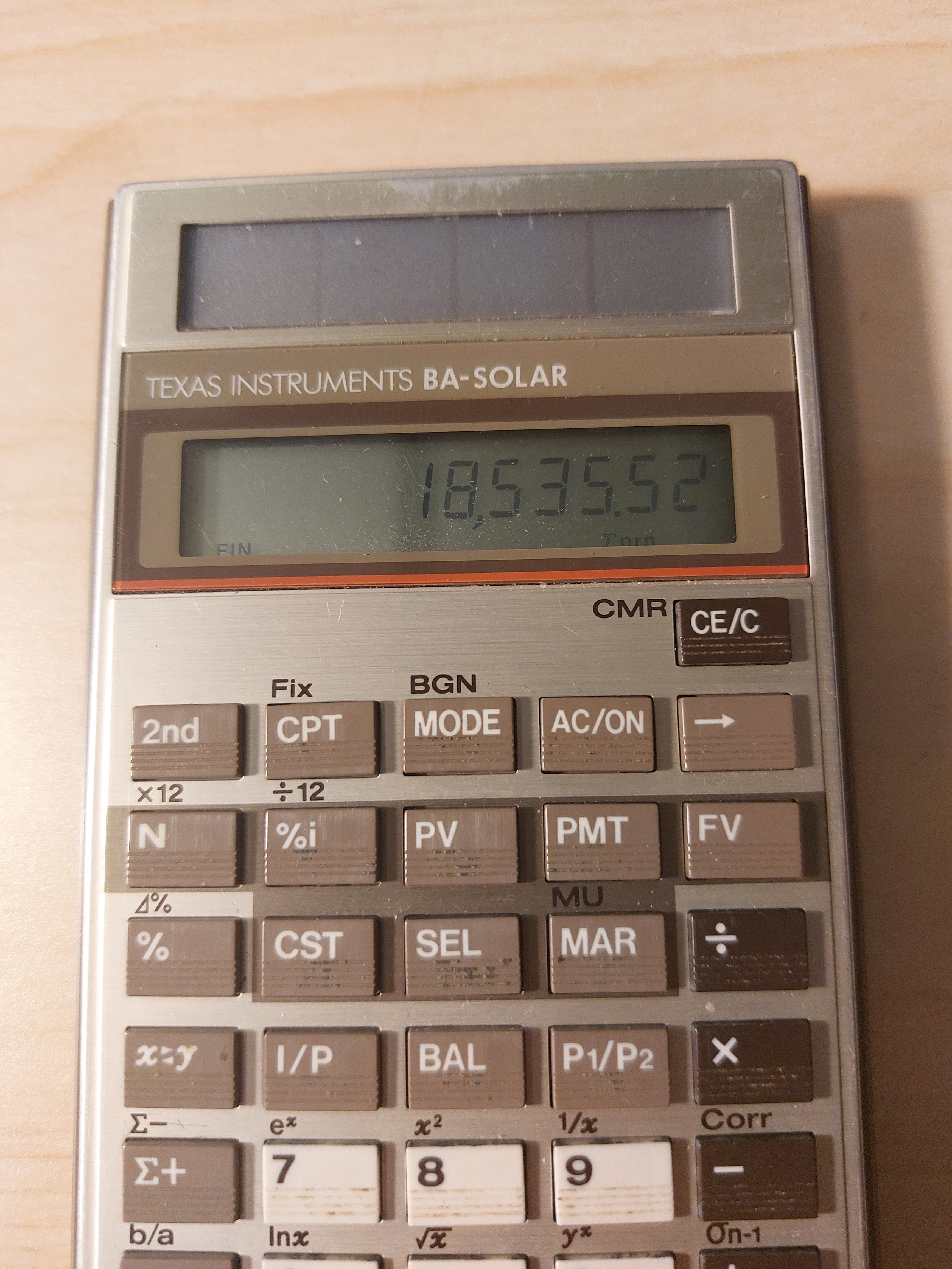
Retro Review: Texas Instruments BA-Solar

Retro Review: Texas Instruments BA-Solar

Finance + Solar + 1980s

Quick Facts

Model:  BA-Solar

Company:  Texas Instruments

Years:  1986 - 1990s; a refresh , BA-35 SOLAR was produced 1996-2000s

Type:  Finance

Batteries: Solar 

Operating Modes:  Chain

Number of Registers: 1, |MEM|

Display:  1 line, 10 digits

Features

The [ MODE ] key is used to toggle between three modes:

FIN Mode:  Time Value of Money  (FIN indicator)

N:  number of payments

%i:  periodic interest rate

PV:  present value

PMT:  payment

FV:  future value

The current cash flow convention is not used, instead the following equation is (I think) used in solving time value of money calculations: 

PV = FV *  SPPV + PMT * USPV

SPPV = single present value factor

USPV = present value annuity factor

We also have amortization functions:

BAL:  balance after any payment

I/P:  interest and principal at any payment

payment_1 P1/P2 payment_2 I/P:  cumulative interest and principal

There are ×12 and ÷12 aids, but we still have to press [ N ] and [ %i ] to register the values, they are not automatic.  

STAT Mode:  Statistics  (STAT indicator)

The BA-SOLAR (and the later BA-35 SOLAR) has both single variable statistics and linear regression.

In linear regression, use the [x<>y] key to change between x and y.   The key will also be used to switch between results.  

Prediction values can be calculated with x' and y'.

The equation used for linear regression is y = a*x + b,  a = slope, b = intercept.

Profit Mode (no indicator)

The profit mode makes the following solver available:

CST:  cost

SEL:  sell

MAR:  margin

MU:  markup

Functions Available in All Modes

Percent Calculations (%):

Add %:  x [ + ] y [ % ] [ = ]

Subtract %:  x [ - ] y [ % ] [ = ]

Multiply %:  x [ × ] y [ % ] [ = ]

Percent Ratio:  part [ ÷ ] whole [ % ] [ = ]

Percent Change:  new [ 2nd ] ( ⊿% ) old [ = ]

rate >EFF payments/year:  convert to effective rate

rate >APR payments/year:  convert to APR/nominal rate

Mathematics:

Natural logarithm and antilogarithm:  ln x, ^x

Square and square root

Power

Reciprocal

Final Thoughts

This is a great basic financial calculator.  I have both the BA-SOLAR and BA-35 SOLAR.   To be honest, I like the keyboard of the original BA-SOLAR better, the keys feel a bit more solid and responsive.  Even though they are no longer in production, the BA-SOLAR is still reasonably available on sites such as eBay and other online stores.  

Source:

Woerner, Joerg.  "Texas Instruments BA-SOLAR"  Last Updated December 5, 2001.   http://www.datamath.org/Sci/Modern/BA-SOLAR.htm   Retrieved May 19, 2022.

Eddie

All original content copyright, © 2011-2022.  Edward Shore.   Unauthorized use and/or unauthorized distribution for commercial purposes without express and written permission from the author is strictly prohibited.  This blog entry may be distributed for noncommercial purposes, provided that full credit is given to the author.