Tampilkan postingan dengan label Python. Tampilkan semua postingan

Matrices in Python without Numpy: Part 4

Matrices in Python without Numpy:  Part 4


We have a good set of tools through out the first three parts.  


For today's blog, let mat1 = [ [ 2, -3, 4 ], [ 1, 5, 7 ] [ 4, 8, -6 ] ]


Screenshots are made using an emulator on my.numworks.com. 


Row Multiply and Add


rowop(matrix, row1, scalar, row2)


Multiplies row1 by a scalar and adds the results to row2.  The matrix is permanently changed.


def rowop(M,r1,s,r2):

  c=len(M[0])

  MT=M

  for k in range (c):

    MT[r2][k]=MT[r1][k]*s+MT[r2][k]

  return MT


Upper Triangle Matrix


utri(matrix)


Changes the matrix to an upper triangular form.  All the elements below the diagonals are zero.  Due to the algorithm, row 0 cannot have a zero or an error occurs.  The algorithm is not perfect.  


def utri(M):

  MT=M

  c=len(M[0])

  for j in range(c-1):

    for k in range(j+1,c):

      rowop(MT,j,-MT[k][j]/MT[j][j],k)

  return MT


Determinant Using the Upper Triangle Matrix


det(matrix)


Calculates the determinant by first transforming the matrix into an upper triangle matrix.


def det(M):

  MT=utri(M)

  d=1

  for k in range(len(MT[0])):

    d*=MT[k][k]

  return d


Please be aware that floating point limitations of Python. 


The determinant should be -322. 


This concludes the series.  


Happy computing,


Eddie 


Source:


Ives, Thom.  "BASIC Linear Algebra Tools in Pure Python without Numpy or Scipy"  Integrated Machine Learning & AI  December 11, 2018.  https://integratedmlai.com/basic-linear-algebra-tools-in-pure-python-without-numpy-or-scipy/


All original content copyright, © 2011-2022.  Edward Shore.   Unauthorized use and/or unauthorized distribution for commercial purposes without express and written permission from the author is strictly prohibited.  This blog entry may be distributed for noncommercial purposes, provided that full credit is given to the author. 


Matrices in Python without Numpy: Part 3

Matrices in Python without Numpy:  Part 3


Today's functions will focus on exact calculations for determinants and inverses for certain sizes:  2 x 2 and 3 x3.  


In the following examples:


mat2 = [ [ 11, 2 ] , [ -8, 4 ] ]

mat3 = [ [ 11, 2, 3 ], [ 4, 51, 6 ], [ 17, 8, 19 ] ]


Screenshots are made using an emulator on my.numworks.com. 


Determinants


det2(matrix):  determinant of a 2 x 2 matrix

det3(matrix):  determinant of a 3 x 3 matrix


def det2(M):

  if len(M)==2 and len(M[0])==2:

    return M[0][0]*M[1][1]-M[0][1]*M[1][0]

  else:

    return "not a 2 x 2 matrix"


def det3(M):

  if len(M)==3 and len(M[0])==3:

    m10=M[1][0]

    m20=M[2][0]

    m11=M[1][1]

    m21=M[2][1]

    m12=M[1][2]

    m22=M[2][2]

    t=M[0][0]*det2([[m11,m12],[m21,m22]])

    t-=M[0][1]*det2([[m10,m12],[m20,m22]])

    t+=M[0][2]*det2([[m10,m11],[m20,m21]])

    return t

  else:

    return "not a 3 x 3 matrix"


Inverses


inv2(matrix):  inverse of a 2 x 2 matrix

inv3(matrix):  inverse of a 3 x 3 matrix


def inv2(M):

  if len(M)==2 and len(M[0])==2:

    MT=newmatrix(2,2)

    t=det2(MT)

    MT[0][0]=M[0][0]*1/t

    MT[0][1]=-M[1][0]*1/t

    MT[1][0]=-M[0][1]*1/t

    MT[1][1]=M[1][1]*1/t

    return MT

  else:

    "not a 2 x 2 matrix"


def inv3(M):

  if len(M)==3 and len(M[0])==3:

    t=det3(M)

    A=newmatrix(3,3)

    A[0][0]=det2([[M[1][1],M[1][2]],[M[2][1],M[2][2]]])/t

    A[0][1]=det2([[M[0][2],M[0][1]],[M[2][2],M[2][1]]])/t

    A[0][2]=det2([[M[0][1],M[0][2]],[M[1][1],M[1][2]]])/t

    A[1][0]=det2([[M[1][2],M[1][0]],[M[2][2],M[2][0]]])/t

    A[1][1]=det2([[M[0][0],M[0][2]],[M[2][0],M[2][2]]])/t

    A[1][2]=det2([[M[0][2],M[0][0]],[M[1][2],M[1][0]]])/t

    A[2][0]=det2([[M[1][0],M[1][1]],[M[2][0],M[2][1]]])/t

    A[2][1]=det2([[M[0][1],M[0][0]],[M[2][1],M[2][0]]])/t

    A[2][2]=det2([[M[0][0],M[0][1]],[M[1][0],M[1][1]]])/t

    return A

  else:

    "not a 3 x 3 matrix"


The functions inv2, inv3, and det3 require det2.  I am using mprint to print matrices as they are supposed to appear.  Please see the blog post on October 3 for the code for mprint. 


Coming up in Part 4, row operations, upper triangular matrices, and determinants of matrices of any size. 


Happy computing,


Eddie 


Source:


Ives, Thom.  "BASIC Linear Algebra Tools in Pure Python without Numpy or Scipy"  Integrated Machine Learning & AI  December 11, 2018.  https://integratedmlai.com/basic-linear-algebra-tools-in-pure-python-without-numpy-or-scipy/


All original content copyright, © 2011-2022.  Edward Shore.   Unauthorized use and/or unauthorized distribution for commercial purposes without express and written permission from the author is strictly prohibited.  This blog entry may be distributed for noncommercial purposes, provided that full credit is given to the author. 


Matrices in Python without Numpy: Part 2

Matrices in Python without Numpy:  Part 2


Let's continue from yesterday.  


Screenshots are made using an emulator on my.numworks.com. 


Matrix Addition


madd(matrix 1, matrix 2)


Adds matrix 1 to matrix 2.  The dimensions of both matrices must be the same.


def madd(A,B):

  # dimension check

  if len(A) != len(B) or len(A[0]) != len(B[0]):

    return "Dimensions of A and B mismatch"

  else:

    M=newmatrix(len(A),len(A[0]))

    for i in range(len(A)):

      for j in range(len(A[0])):

        M[i][j]=A[i][j]+B[i][j]

    return M


In this example screen shot:


mat1 = [ [ 8, -2 ], [ -4, 7 ] ]

mat2 = [ [ 1, 3 ], [ 5, 6 ] ]


Matrix addition is communitive.  Hence,  mat1 + mat2 = mat2 + mat1.


Matrix Multiplication


mmult(mat1, mat2)


Multiplies mat1 to mat2.  Here the number of columns of mat1 must be the same as the rows of mat2.  


Matrix multiplication is not communitive.  Hence, mat1 * mat2 ≠ mat2 * mat1


def mmult(A,B):

  # dimension check

  if len(A[0]) != len(B):

    return "Columns of A != Rows of B"

  else:

    M=newmatrix(len(A),len(B[0]))

    for i in range(len(A)):

      for j in range(len(B[0])):

        t=0

        for k in range(len(A[0])):

          t +=A[i][k]*B[k][j]

        M[i][j]=t

    return M


Note that both madd and mmult require newmatrix.  See yesterday's post for the code for newmatrix. 


Next time, we will work with determinants and inverses.


Happy computing,


Eddie 


Source:


Ives, Thom.  "BASIC Linear Algebra Tools in Pure Python without Numpy or Scipy"  Integrated Machine Learning & AI  December 11, 2018.  https://integratedmlai.com/basic-linear-algebra-tools-in-pure-python-without-numpy-or-scipy/


All original content copyright, © 2011-2022.  Edward Shore.   Unauthorized use and/or unauthorized distribution for commercial purposes without express and written permission from the author is strictly prohibited.  This blog entry may be distributed for noncommercial purposes, provided that full credit is given to the author. 


Matrices in Python without Numpy: Part 1

Matrices in Python without Numpy:  Part 1


Introduction


Python is a wonderful programming language and is a welcome addition to graphing calculators such as:


*  TI nSpire CX II  and TI nSpire CX II CAS

*  TI-84 Plus CE Python (it's become hard to find and hopefully it won't be the case in 2023)

*  HP Prime

*  Casio fx-CG 50

*  Casio fx-9750GIII and fx-9860GIII

*  Numworks

*  From France:  TI-83 Premium Python, TI-82 Advanced Edition Python, Casio Graph fx-35+ E II


As I understand at time, there is no numpy module for any of the calculators*.   


But we want to work with matrices.  So we will need to program code to allow work with matrices.  Welcome to the Matrices in Python without Numpy series!


* There is a linalg module for the HP Prime.  


This series will cover:


*  creating matrices and other basics

*  adding and multiplying matrices

*  determinant and inverse of 2 x 2 and 3 x 3 matrices

*  upper triangular matrices and general determinant


In this series, a single Python file is created, matrix.py.   Each of the commands are going to be a separate function within a define structure.   This allows matrix.py to imported into other Python scripts by from matrix import *.  


Entering Matrices


Use square brackets to enter matrices:  


[ [ M11, M12, M13, ... ] , [ M21, M22, M23, ... ] , [ M31, M32, M33, ... ] ] 


Each row enclosing elements per column, and each row is separated by a comma.  All the rows are enclosed in square brackets.  


In this sense, matrices in this sense are nested lists.  Call elements by:


Call a row:   matrix[row]

Call the last row:  matrix[-1]

Call an element:  matrix[row][column]


Number of rows:  len(matrix)

Number of columns:  len(matrix[0])


Remember, in Python, indices start with 0 and go to row-1, column-1.  We will stick with the index convention to stay consistent.  


Screenshots are made using an emulator on my.numworks.com


Creating and Printing Matrices


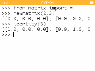
newmatrix(number of rows, number of columns).  


The matrix will be filled with zeros.


Code:

def newmatrix(r,c):

  M = []

  while len(M)<r:

    M.append([])

    while len(M[-1])<c:

      M[-1].append(0.0)

  return M


identity(size)


Creates an identity matrix, a square matrix with ones in the diagonal, zeroes everywhere else.  The identity matrix a fundamental matrix.


Code:


def identity(n):

  M = newmatrix(n,n)

  for i in range(n):

    M[i][i]=1.0

  return M


So far, we see resulting matrices in a row or scroll off the screen.  Let's make it so we can see matrices as they are written.  


mprint(matrix)


Prints a matrix in text form.


def mprint(M):

  for r in M:

    print([x+0 for x in r])


List comprehension is a very powerful tool in Python.


In the following examples, we will store a 3 x 3 matrix:


mat1 = [ [ 1, 2, 3 ] , [ 4, 5, 6 ] , [ 7, 8, 9 ] ] 


transpose(matrix)


The transpose function flips a matrix on it's diagonal.  For each element:


M^T:   M(row, col) → M^T(col, row)


def transpose(M):

  # get numbers of rows

  r=len(M)

  # get number of columns

  c=len(M[0])

  # create transpose matrix

  MT=newmatrix(c,r)

  for i in range(r):

    for j in range(c):

      MT[j][i]=M[i][j]

  return MT


scalar(matrix, factor)


Next, we have scalar multiplication, multiply each element of the matrix by the factor.


def scalar(M,s):

  r=len(M)

  c=len(M[0])

  MT=newmatrix(r,c)

  for i in range(r):

    for j in range(c):

      MT[i][j]=s*M[i][j]

  return MT


mtrace(matrix)


Finally, we have the a trace of a matrix.  The trace is the sum of all the diagonals of a square matrix.  If the matrix is not square, an error occurs.


def mtrace(M):

  r=len(M)

  c=len(M[0])

  MT=newmatrix(r,c)

  if r !=c:

    return "Not a square matrix"

  else:

    t=0

    for i in range(r):

      t+=M[i][i]

    return t


In Python != means not equal.  


Coming in Part 2, let's add and multiply matrices.  


Happy computing,


Eddie 


Source:


Ives, Thom.  "BASIC Linear Algebra Tools in Pure Python without Numpy or Scipy"  Integrated Machine Learning & AI  December 11, 2018.  https://integratedmlai.com/basic-linear-algebra-tools-in-pure-python-without-numpy-or-scipy/


All original content copyright, © 2011-2022.  Edward Shore.   Unauthorized use and/or unauthorized distribution for commercial purposes without express and written permission from the author is strictly prohibited.  This blog entry may be distributed for noncommercial purposes, provided that full credit is given to the author. 


TI 84 Plus CE TI-Basic and TI Nspire CX II Python: Gamma by Multiplication Recursion Property

TI 84 Plus CE TI-Basic and TI Nspire CX II Python:   Gamma by Multiplication Recursion Property


Introduction


The program calculates the gamma function for any real positive number in tenths by the multiplication recursion:


Γ(x + 1) = x * Γ(x)


For example:  


Γ(2.5)

= 1.5 * Γ(1.5)

= 1.5 * 0.5 * Γ(0.5)

≈ 1.5 * 0.5 * 1.772453851

≈ 1.329340388


Reduce x by 1 until 1 is in between 0.1 and 1. 


Gamma Values:


Γ(0.1) = 9.513507699

Γ(0.2) = 4.590843712

Γ(0.3) = 2.991568988

Γ(0.4) = 2.218159544

Γ(0.5) = 1.772453851

Γ(0.6) = 1.489192249

Γ(0.7) = 1.298055333

Γ(0.8) = 1.164229714

Γ(0.9) = 1.068628702

Γ(1) = 1


TI-84 Plus CE Program: GAMMATEN

TI-Basic


Notes:


*  To get the small L to create lists with custom names, get the character with the key strokes:  [ 2nd ] ( list ), OPS, B.  L.   In this listing, I will write L^ to symbolize the lower case L.


* L^TEN is a custom list.


Program listing:


{9.513507699, 4.590843712, 2.991568988, 

2.218159544, 1.772453851, 1.489192249,

1.298055333, 1.164229714, 1.068628702

1}→L^TEN

ClrHome

Disp "GAMMA X (NEAREST 0.1)"

Input "X≥0.1, X?",X

round(X,1)→X

fPart(X)*10→F

If F=0:10→F

1→G

While X>1

G*(X-1)→G

X-1→X

End

G*L^TEN(F)→G

Disp "EST. GAMMA: ", G


TI-NSpire Python Script:  gammaten.py


The code is defined as a function.   


def gammaten(x):

  lten=[9.513507699]

  lten.append(4.590843712)

  lten.append(2.991568988)

  lten.append(2.218159544)

  lten.append(1.772453851)

  lten.append(1.489192249)

  lten.append(1.298055333)

  lten.append(1.164229714)

  lten.append(1.068628702)

  lten.append(1)

  #print("gamma(x) to the nearest 0.1")

  x=round(x,1)

  f=round(10*(x-int(x))-1)

  g=1

  while x>1:

    x-=1

    g*=x

  g*=lten[f]

  return [g,f]


# list[-1] gets last item too

# round integers for accurate results!

# 2022-06-13 EWS


Eddie 


All original content copyright, © 2011-2022.  Edward Shore.   Unauthorized use and/or unauthorized distribution for commercial purposes without express and written permission from the author is strictly prohibited.  This blog entry may be distributed for noncommercial purposes, provided that full credit is given to the author. 


Python - Lambda Week: Solving Differential Equations with Runge Kutta 4th Order Method

Python - Lambda Week: Solving Differential Equations with Runge Kutta 4th Order Method


Welcome to Python Week!  This we we're going to cover calculus and the keyword lambda.


Note:  All Python scripts presented this week were created using a TI-NSpire CX II CAS.   As of June 2022, the lambda keyword is available on all calculators (in the United States) that have Python.   If you are not sure, please check your calculator manual. 


Solving Differential Equations


This following script solves the differential equation:


y' = dy/dx = f(x,y)

with initial condition y(x0) = y0


Repeat the steps for each step size h:

f1 = h * f(x0, y0)

f2 = h * f(x0 + h/2, y0 + f1/2)

f3 = h * f(x0 + h/2, y0 + f2/2)

f4 = h * f(x0 + h, y0 + f3)

x0 = x0 + h   (update x)

y0 = y0 + (f1 + 2*f2 + 2*f3 + f4)/6   (update y)


The small h is, the more accurate the calculated coordinates are.  


rk4lam.py:  Runge Kutta 4th Order Method


All answers are stored in the nested list t.  


from math import *

print("Runge Kutta 4th Order")

print("Math Module imported")

f=eval("lambda x,y:"+input("dy/dx = "))


# must call for float numbers one at a time

x0=eval(input("x0 = "))

y0=eval(input("y0 = "))

h=eval(input("h = "))


# ask for an integer

n=int(input("number of steps: "))


# set up table

t=[[x0,y0]]


# main loop

for i in range(n):

  f1=h*f(x0,y0)

  f2=h*f(x0+h/2,y0+f1/2)

  f3=h*f(x0+h/2,y0+f2/2)

  f4=h*f(x0+h,y0+f3)

  x0=x0+h

  y0=y0+(f1+2*f2+2*f3+f4)/6

  print([x0,y0])

  t.append([x0,y0])


print("Done.  Recall t for table.")


Examples


Results are rounded to five digits.  


Example 1:

dy/dx = 2*x*y + x,  y(0) = 0, h = 0.1, 5 steps

(Real solution:  y = 1/2 * (e^(x^2) - 1))


Results (which matches the exact results):

x = 0.1, y ≈ 0.00503

x = 0.2, y ≈ 0.02041

x = 0.3, y ≈ 0.04709

x = 0.4, y ≈ 0.08676

x = 0.5, y ≈ 0.14201


Example 2:

dy/dx = ln x + y, y(10) = 1

(Real Solution:  y = [∫(ln t * e^(-t) dt, t = 10 to x) + e^(-10)] * e^x


Exact Results:

x = 11, y ≈ 6.74551

x = 12, y ≈ 22.51732

x = 13, y ≈ 65.53659

x = 14, y ≈ 182.60824

x = 15, y ≈ 500.96552


Runge Kutta with h = 1, 5 steps:

x = 11, y ≈ 6.71066

x = 12, y ≈ 22.33376

x = 13, y ≈ 64.78988

x = 14, y ≈ 179.90761

x = 15, y ≈ 491.80768


Runge Kutta with h = 0.1, 50 steps:

x = 11, y ≈ 6.74551   (recall t[10])

x = 12, y ≈ 22.51728   (t[20])

x = 13, y ≈ 65.53643   (t[30])

x = 14, y ≈ 182.60766  (t[40])

x = 15, y ≈ 500.96358  (t[50])


This ends Python week for now, I hope you find this week helpful and resourceful.


Until next time,


Eddie


All original content copyright, © 2011-2022.  Edward Shore.   Unauthorized use and/or unauthorized distribution for commercial purposes without express and written permission from the author is strictly prohibited.  This blog entry may be distributed for noncommercial purposes, provided that full credit is given to the author. 


Python - Lambda Week: Integration by Simpson's Rule

Python - Lambda Week: Integration by Simpson's Rule


Welcome to Python Week!  This we we're going to cover calculus and the keyword lambda.


Note:  All Python scripts presented this week were created using a TI-NSpire CX II CAS.   As of June 2022, the lambda keyword is available on all calculators (in the United States) that have Python.   If you are not sure, please check your calculator manual. 


Simpson's Rule


The Simpson's Rule estimates numeric integrals by:


∫( f(x) dx, x = a to b) ≈

(b - a) /(3 * n) * (f(a) + 4 * f1 + 2 * f2 + 4 * f3 + .... + 2 * f_n-2 + 4 * f_n-1 + f(b))


n must be an even number of partitions.  The more partitions, the higher the accuracy and the higher computation time.


integrallam.py:  Numeric Integer


from math import *


print("The math module is imported.")

print("Integra of f(x), 6 places")

f=eval("lambda x:"+input("f(x)? "))


# input parameters

a=eval(input("lower = "))

b=eval(input("upper = "))

n=int(input("even parts: "))


# checksafe, add 1 if n is odd

if n/2-int(n/2)==0:

  n=n+1


# integral calculus

s=f(a)+f(b)

w=1

# 1 to n-1

for i in range(1,n):

  w=f(a+i*(b-a)/n)

  s+=(2*w) if (i/2-int(i/2)==0) else (4*w)

s*=(b-a)/(3*n)

print("Integral: "+str(round(s,6)))


All original content copyright, © 2011-2022.  Edward Shore.   Unauthorized use and/or unauthorized distribution for commercial purposes without express and written permission from the author is strictly prohibited.  This blog entry may be distributed for noncommercial purposes, provided that full credit is given to the author. 

Python - Lambda Week: Derivatives and Newton's Method

Python - Lambda Week: Derivatives and Newton's Method


Welcome to Python Week!  This we we're going to cover calculus and the keyword lambda.


Note:  All Python scripts presented this week were created using a TI-NSpire CX II CAS.   As of June 2022, the lambda keyword is available on all calculators (in the United States) that have Python.   If you are not sure, please check your calculator manual. 


Derivative


The Five Stencil Method is used.  Due to the approximate nature, results are rounded to 5 digits.


f'(x) ≈ (-f(x+2*h) + 8*f(x+h) - 8*f(x-h) + f(x-2*h)) / (12 * h)


h is set to 0.0001 to allow for a wide range of functions and to hopefully prevent float point overflows or underflows.  You can modify h or have the user input a value if you so wish.  


derivlam.py:  Derivative Using the Five Stencil Method


# Math Calculations

#================================

from math import *

#================================


print("The math module is imported.")

f=eval("lambda x:"+input("f(x)? "))


# input x0

x=eval(input("d/dx at x0: "))

h=.0001


# derivative, 5 stencil

d=(-f(x+2*h)+8*f(x+h)-8*f(x-h)+f(x-2*h))/(12*h)

print("round to 5 decimal points")

print("d/dx = "+str(round(d,5)))


Newton's Method


The next script finds the root of f(x) (solve f(x) = 0) with a guess.  


x_n+1 = x_n - f(x_n) / f'(x_n)


The derivative is calculated using the Five Stencil Method.   


I put a limit of 100 iterations because Newton's Method is not always perfect nor this script finds solutions in the complex plane, just the real numbers.  


newtonlam.py


# Math Calculations

#================================

from math import *

#================================

print("The math module is imported.")

print("Solve f(x)=0 to 6 places")

f=eval("lambda x:"+input("f(x)? "))


# input x0

x=eval(input("Guess? "))

h=.0001


w=1

n=1

while fabs(w)>10**(-7):

  d=(-f(x+2*h)+8*f(x+h)-8*f(x-h)+f(x-2*h))/(12*h)

  w=f(x)/d

  x-=w

  n+=1

  if n>100:

    print("iterations exceeded")

    break


if n<101:

  print("x = "+str(round(x,6)))

  print("iterations used: "+str(n))


All original content copyright, © 2011-2022.  Edward Shore.   Unauthorized use and/or unauthorized distribution for commercial purposes without express and written permission from the author is strictly prohibited.  This blog entry may be distributed for noncommercial purposes, provided that full credit is given to the author. 


Python - Lambda Week: Plotting Functions

Python - Lambda Week: Plotting Functions


Welcome to Python Week!  This we we're going to cover calculus and the keyword lambda.


Note:  All Python scripts presented this week were created using a TI-NSpire CX II CAS.   As of June 2022, the lambda keyword is available on all calculators (in the United States) that have Python.   If you are not sure, please check your calculator manual. 


Plotting Functions


We can use the line:


f=eval("lambda x:"+input("f(x) = "))


for multiple applications.   Remember, lambda functions are not defined so that they can be used outside of the Python script it belongs to but it lambda functions are super useful!


This code is specific to the Texas Instruments calculators (TI-Nspire CX II (CAS), TI-84 Plus CE Python, TI-83 CE Premium Python Edition, but NOT the TI-82 Advanced Python).    For other calculators, HP Prime, Casio fx-CG 50, Casio fx-9750GIII/9860GIII, Numworks, or computer Python, apply similar language. 


plotlam.py:  Plotting with Lambda


from math import *

import ti_plotlib as plt


# this is for the TI calcs

# other calculators will use their own plot syntax


print("The math module is imported.")

# input defaults to string

# use the plus sign to combine strings

f=eval("lambda x:"+input("f(x) = "))


# set up parameters

x0=eval(input("x min = "))

x1=eval(input("x max = "))


# we want n to be an integer

n=int(input("number of points = "))


# calculate step size

h=(x1-x0)/n


# calculate plot lists

x=[]

y=[]

i=x0

while i<=x1:

  x.append(i)

  y.append(f(i))

  i+=h


# choose color (not for Casio fx-9750/9850GIII)

# colors are defined using tuples

colors=((0,0,0),(255,0,0),(0,128,0),(0,0,255))

print("0: black \n1: red \n2: green \n3: blue")

c=int(input("Enter a color code: "))


# plot f(x)

# auto setup to x and y lists

plt.auto_window(x,y)


# plot axes

plt.color(128,128,128)

plt.axes("axes")


# plot the function

plt.color(colors[c])

plt.plot(x,y,".")

plt.show_plot()


All original content copyright, © 2011-2022.  Edward Shore.   Unauthorized use and/or unauthorized distribution for commercial purposes without express and written permission from the author is strictly prohibited.  This blog entry may be distributed for noncommercial purposes, provided that full credit is given to the author. 


Python - Lambda Week: Building and Asking for Functions

Python - Lambda Week: Building and Asking for Functions


Welcome to Python Week!  This we we're going to cover calculus and the keyword lambda.


Note:  All Python scripts presented this week were created using a TI-NSpire CX II CAS.   As of June 2022, the lambda keyword is available on all calculators (in the United States) that have Python.   If you are not sure, please check your calculator manual. 


Lambda - Introduction


The key word lambda allows us to define a one-line function in Python program for internal use.  Keep in mind, this is different from the define (def-return) structure, where we can define multiline functions and can be used to be imported into other programs or the shell.


I briefly introduced lambda last September:  https://edspi31415.blogspot.com/2021/09/calculator-python-lambda-functions.html


The syntax for lambda is for one argument:


fx=lambda var:define f(var) here


And we can use fx(var) to calculate the lambda function. 


We can use more than one argument, and the syntax looks something like this:


fx=lambda var1, var2, ...:define f(var1, var2, ...)


We use fx(var1,var2,...) to recall and calculate.


Keep in mind, a lambda function can accept many arguments, but can only return one answer.   The script lambdabuild.py shows a short demonstration of the lamdba key word:


lambdabuild.py:   Build a lambda function


from math import *

#================================

# build a lambda function


fx=lambda x:x**2+1

print("x=1, ",str(fx(1)))

print("x=2, ",str(fx(2)))


# lambda can have more than 1 input, but 

# must have only 1 output


gxy=lambda x,y:sqrt(x**2+y**2)

print("x=3, y=4",str(gxy(3,4)))

print("x=6, y=10",str(gxy(6,10)))


Getting User Input


We can ask for a user function by the lines:

fs=input("text here")

fx=eval("lambda var:"+fs)


This can be combined in one line:

fx=eval("lambda var:"+input("prompt"))


For example:

fx=eval("lambda x:"+input("f(x) = "))


The eval function changes a string to an expression to be evaluated.  This is great because we can use eval to change strings to make lambda functions and ask for input of numerical expressions including pi (assuming the math module is imported).


lambda2.py:   Asking for a function


# Math Calculations

#================================

from math import *

#================================

# ask the user to define a function

# input defaults as a string


print("The math module is imported.")

print("Use eval for allow for numeric expressions,")

print("including pi.")

f=eval("lambda x:"+input("f(x) = "))


# ask for three inputs

# use eval to allow for expressions

x1=eval(input("x1? "))

x2=eval(input("x2? "))

x3=eval(input("x3? "))


# calculate

y1=f(x1)

y2=f(x2)

y3=f(x3)


# print results

print("Here are your results:")

print(x1, y1)

print(x2, y2)

print(x3, y3)


All original content copyright, © 2011-2022.  Edward Shore.   Unauthorized use and/or unauthorized distribution for commercial purposes without express and written permission from the author is strictly prohibited.  This blog entry may be distributed for noncommercial purposes, provided that full credit is given to the author. 


Backlink 9999 Traffic Super

Order Now...!!!!