Python - Lambda Week: Solving Differential Equations with Runge Kutta 4th Order Method

Python - Lambda Week: Solving Differential Equations with Runge Kutta 4th Order Method

Welcome to Python Week!  This we we're going to cover calculus and the keyword lambda.

Note:  All Python scripts presented this week were created using a TI-NSpire CX II CAS.   As of June 2022, the lambda keyword is available on all calculators (in the United States) that have Python.   If you are not sure, please check your calculator manual. 

Solving Differential Equations

This following script solves the differential equation:

y' = dy/dx = f(x,y)

with initial condition y(x0) = y0

Repeat the steps for each step size h:

f1 = h * f(x0, y0)

f2 = h * f(x0 + h/2, y0 + f1/2)

f3 = h * f(x0 + h/2, y0 + f2/2)

f4 = h * f(x0 + h, y0 + f3)

x0 = x0 + h   (update x)

y0 = y0 + (f1 + 2*f2 + 2*f3 + f4)/6   (update y)

The small h is, the more accurate the calculated coordinates are.  

rk4lam.py:  Runge Kutta 4th Order Method

All answers are stored in the nested list t.  

from math import *

print("Runge Kutta 4th Order")

print("Math Module imported")

f=eval("lambda x,y:"+input("dy/dx = "))

# must call for float numbers one at a time

x0=eval(input("x0 = "))

y0=eval(input("y0 = "))

h=eval(input("h = "))

# ask for an integer

n=int(input("number of steps: "))

# set up table

t=[[x0,y0]]

# main loop

for i in range(n):

  f1=h*f(x0,y0)

  f2=h*f(x0+h/2,y0+f1/2)

  f3=h*f(x0+h/2,y0+f2/2)

  f4=h*f(x0+h,y0+f3)

  x0=x0+h

  y0=y0+(f1+2*f2+2*f3+f4)/6

  print([x0,y0])

  t.append([x0,y0])

print("Done.  Recall t for table.")

Examples

Results are rounded to five digits.  

Example 1:

dy/dx = 2*x*y + x,  y(0) = 0, h = 0.1, 5 steps

(Real solution:  y = 1/2 * (e^(x^2) - 1))

Results (which matches the exact results):

x = 0.1, y ≈ 0.00503

x = 0.2, y ≈ 0.02041

x = 0.3, y ≈ 0.04709

x = 0.4, y ≈ 0.08676

x = 0.5, y ≈ 0.14201

Example 2:

dy/dx = ln x + y, y(10) = 1

(Real Solution:  y = [∫(ln t * e^(-t) dt, t = 10 to x) + e^(-10)] * e^x

Exact Results:

x = 11, y ≈ 6.74551

x = 12, y ≈ 22.51732

x = 13, y ≈ 65.53659

x = 14, y ≈ 182.60824

x = 15, y ≈ 500.96552

Runge Kutta with h = 1, 5 steps:

x = 11, y ≈ 6.71066

x = 12, y ≈ 22.33376

x = 13, y ≈ 64.78988

x = 14, y ≈ 179.90761

x = 15, y ≈ 491.80768

Runge Kutta with h = 0.1, 50 steps:

x = 11, y ≈ 6.74551   (recall t[10])

x = 12, y ≈ 22.51728   (t[20])

x = 13, y ≈ 65.53643   (t[30])

x = 14, y ≈ 182.60766  (t[40])

x = 15, y ≈ 500.96358  (t[50])

This ends Python week for now, I hope you find this week helpful and resourceful.

Until next time,

Eddie

All original content copyright, © 2011-2022.  Edward Shore.   Unauthorized use and/or unauthorized distribution for commercial purposes without express and written permission from the author is strictly prohibited.  This blog entry may be distributed for noncommercial purposes, provided that full credit is given to the author. 

Python - Lambda Week: Integration by Simpson's Rule

Python - Lambda Week: Integration by Simpson's Rule

Welcome to Python Week!  This we we're going to cover calculus and the keyword lambda.

Note:  All Python scripts presented this week were created using a TI-NSpire CX II CAS.   As of June 2022, the lambda keyword is available on all calculators (in the United States) that have Python.   If you are not sure, please check your calculator manual. 

Simpson's Rule

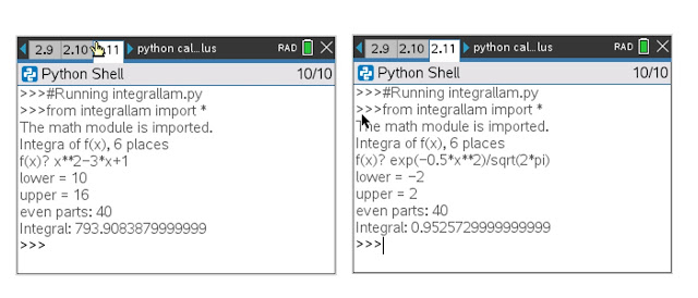
The Simpson's Rule estimates numeric integrals by:

∫( f(x) dx, x = a to b) ≈

(b - a) /(3 * n) * (f(a) + 4 * f1 + 2 * f2 + 4 * f3 + .... + 2 * f_n-2 + 4 * f_n-1 + f(b))

n must be an even number of partitions.  The more partitions, the higher the accuracy and the higher computation time.

integrallam.py:  Numeric Integer

from math import *

print("The math module is imported.")

print("Integra of f(x), 6 places")

f=eval("lambda x:"+input("f(x)? "))

# input parameters

a=eval(input("lower = "))

b=eval(input("upper = "))

n=int(input("even parts: "))

# checksafe, add 1 if n is odd

if n/2-int(n/2)==0:

  n=n+1

# integral calculus

s=f(a)+f(b)

w=1

# 1 to n-1

for i in range(1,n):

  w=f(a+i*(b-a)/n)

  s+=(2*w) if (i/2-int(i/2)==0) else (4*w)

s*=(b-a)/(3*n)

print("Integral: "+str(round(s,6)))

All original content copyright, © 2011-2022.  Edward Shore.   Unauthorized use and/or unauthorized distribution for commercial purposes without express and written permission from the author is strictly prohibited.  This blog entry may be distributed for noncommercial purposes, provided that full credit is given to the author. 

Python - Lambda Week: Derivatives and Newton's Method

Python - Lambda Week: Derivatives and Newton's Method

Welcome to Python Week!  This we we're going to cover calculus and the keyword lambda.

Note:  All Python scripts presented this week were created using a TI-NSpire CX II CAS.   As of June 2022, the lambda keyword is available on all calculators (in the United States) that have Python.   If you are not sure, please check your calculator manual. 

Derivative

The Five Stencil Method is used.  Due to the approximate nature, results are rounded to 5 digits.

f'(x) ≈ (-f(x+2*h) + 8*f(x+h) - 8*f(x-h) + f(x-2*h)) / (12 * h)

h is set to 0.0001 to allow for a wide range of functions and to hopefully prevent float point overflows or underflows.  You can modify h or have the user input a value if you so wish.  

derivlam.py:  Derivative Using the Five Stencil Method

# Math Calculations

#================================

from math import *

#================================

print("The math module is imported.")

f=eval("lambda x:"+input("f(x)? "))

# input x0

x=eval(input("d/dx at x0: "))

h=.0001

# derivative, 5 stencil

d=(-f(x+2*h)+8*f(x+h)-8*f(x-h)+f(x-2*h))/(12*h)

print("round to 5 decimal points")

print("d/dx = "+str(round(d,5)))

Newton's Method

The next script finds the root of f(x) (solve f(x) = 0) with a guess.  

x_n+1 = x_n - f(x_n) / f'(x_n)

The derivative is calculated using the Five Stencil Method.   

I put a limit of 100 iterations because Newton's Method is not always perfect nor this script finds solutions in the complex plane, just the real numbers.  

newtonlam.py

# Math Calculations

#================================

from math import *

#================================

print("The math module is imported.")

print("Solve f(x)=0 to 6 places")

f=eval("lambda x:"+input("f(x)? "))

# input x0

x=eval(input("Guess? "))

h=.0001

w=1

n=1

while fabs(w)>10**(-7):

  d=(-f(x+2*h)+8*f(x+h)-8*f(x-h)+f(x-2*h))/(12*h)

  w=f(x)/d

  x-=w

  n+=1

  if n>100:

    print("iterations exceeded")

    break

if n<101:

  print("x = "+str(round(x,6)))

  print("iterations used: "+str(n))

All original content copyright, © 2011-2022.  Edward Shore.   Unauthorized use and/or unauthorized distribution for commercial purposes without express and written permission from the author is strictly prohibited.  This blog entry may be distributed for noncommercial purposes, provided that full credit is given to the author. 

Python - Lambda Week: Plotting Functions

Python - Lambda Week: Plotting Functions

Welcome to Python Week!  This we we're going to cover calculus and the keyword lambda.

Note:  All Python scripts presented this week were created using a TI-NSpire CX II CAS.   As of June 2022, the lambda keyword is available on all calculators (in the United States) that have Python.   If you are not sure, please check your calculator manual. 

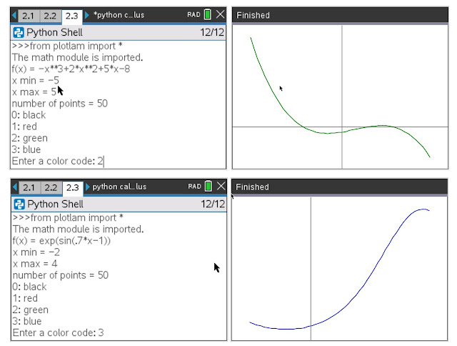
Plotting Functions

We can use the line:

f=eval("lambda x:"+input("f(x) = "))

for multiple applications.   Remember, lambda functions are not defined so that they can be used outside of the Python script it belongs to but it lambda functions are super useful!

This code is specific to the Texas Instruments calculators (TI-Nspire CX II (CAS), TI-84 Plus CE Python, TI-83 CE Premium Python Edition, but NOT the TI-82 Advanced Python).    For other calculators, HP Prime, Casio fx-CG 50, Casio fx-9750GIII/9860GIII, Numworks, or computer Python, apply similar language. 

plotlam.py:  Plotting with Lambda

from math import *

import ti_plotlib as plt

# this is for the TI calcs

# other calculators will use their own plot syntax

print("The math module is imported.")

# input defaults to string

# use the plus sign to combine strings

f=eval("lambda x:"+input("f(x) = "))

# set up parameters

x0=eval(input("x min = "))

x1=eval(input("x max = "))

# we want n to be an integer

n=int(input("number of points = "))

# calculate step size

h=(x1-x0)/n

# calculate plot lists

x=[]

y=[]

i=x0

while i<=x1:

  x.append(i)

  y.append(f(i))

  i+=h

# choose color (not for Casio fx-9750/9850GIII)

# colors are defined using tuples

colors=((0,0,0),(255,0,0),(0,128,0),(0,0,255))

print("0: black \n1: red \n2: green \n3: blue")

c=int(input("Enter a color code: "))

# plot f(x)

# auto setup to x and y lists

plt.auto_window(x,y)

# plot axes

plt.color(128,128,128)

plt.axes("axes")

# plot the function

plt.color(colors[c])

plt.plot(x,y,".")

plt.show_plot()

All original content copyright, © 2011-2022.  Edward Shore.   Unauthorized use and/or unauthorized distribution for commercial purposes without express and written permission from the author is strictly prohibited.  This blog entry may be distributed for noncommercial purposes, provided that full credit is given to the author. 

Python - Lambda Week: Building and Asking for Functions

Python - Lambda Week: Building and Asking for Functions

Welcome to Python Week!  This we we're going to cover calculus and the keyword lambda.

Note:  All Python scripts presented this week were created using a TI-NSpire CX II CAS.   As of June 2022, the lambda keyword is available on all calculators (in the United States) that have Python.   If you are not sure, please check your calculator manual. 

Lambda - Introduction

The key word lambda allows us to define a one-line function in Python program for internal use.  Keep in mind, this is different from the define (def-return) structure, where we can define multiline functions and can be used to be imported into other programs or the shell.

I briefly introduced lambda last September:  https://edspi31415.blogspot.com/2021/09/calculator-python-lambda-functions.html

The syntax for lambda is for one argument:

fx=lambda var:define f(var) here

And we can use fx(var) to calculate the lambda function. 

We can use more than one argument, and the syntax looks something like this:

fx=lambda var1, var2, ...:define f(var1, var2, ...)

We use fx(var1,var2,...) to recall and calculate.

Keep in mind, a lambda function can accept many arguments, but can only return one answer.   The script lambdabuild.py shows a short demonstration of the lamdba key word:

lambdabuild.py:   Build a lambda function

from math import *

#================================

# build a lambda function

fx=lambda x:x**2+1

print("x=1, ",str(fx(1)))

print("x=2, ",str(fx(2)))

# lambda can have more than 1 input, but 

# must have only 1 output

gxy=lambda x,y:sqrt(x**2+y**2)

print("x=3, y=4",str(gxy(3,4)))

print("x=6, y=10",str(gxy(6,10)))

Getting User Input

We can ask for a user function by the lines:

fs=input("text here")

fx=eval("lambda var:"+fs)

This can be combined in one line:

fx=eval("lambda var:"+input("prompt"))

For example:

fx=eval("lambda x:"+input("f(x) = "))

The eval function changes a string to an expression to be evaluated.  This is great because we can use eval to change strings to make lambda functions and ask for input of numerical expressions including pi (assuming the math module is imported).

lambda2.py:   Asking for a function

# Math Calculations

#================================

from math import *

#================================

# ask the user to define a function

# input defaults as a string

print("The math module is imported.")

print("Use eval for allow for numeric expressions,")

print("including pi.")

f=eval("lambda x:"+input("f(x) = "))

# ask for three inputs

# use eval to allow for expressions

x1=eval(input("x1? "))

x2=eval(input("x2? "))

x3=eval(input("x3? "))

# calculate

y1=f(x1)

y2=f(x2)

y3=f(x3)

# print results

print("Here are your results:")

print(x1, y1)

print(x2, y2)

print(x3, y3)

All original content copyright, © 2011-2022.  Edward Shore.   Unauthorized use and/or unauthorized distribution for commercial purposes without express and written permission from the author is strictly prohibited.  This blog entry may be distributed for noncommercial purposes, provided that full credit is given to the author. 

Casio fx-CG50: Sparse Matrix Builder

Casio fx-CG50: Sparse Matrix Builder

Introduction

The programs can create a sparse matrix, a matrix where most of the entries have zero value.  There are several ways to represent sparse matrix in a shortcut form.  The most straight forward way is the COO (row-column-value) representation.

Mat A:  three column matrix:  (row-column-value representation)

Column 1:  row number

Column 2:  column number

Column 3:  value

Mat S:  sparse matrix

Casio fx-CG 50 Program:  SPARSE

[ [ row, column, value ] ... ] → sparse matrix

"TO SPARSE MATRIX"

"EDWARD SHORE"

"[[ROW,COL,VALUE]]"

"MAT"?→Mat A

Mat→List(Mat A,1)→List 26

Max(List 26)→R

Mat→List(Mat A,2)→List 26

Max(List 26)→C

{R,C}→Dim Mat S

Dim Mat A→List 26

List 26[1]→N

For 1→I To N

Mat A[I,1]→J

Mat A[I,2]→K

Mat A[I,3]→Mat S[J,K]

Next 

"SPARSE MATRIX:"⊿

Mat S

Casio fx-CG 50 Program: ISPARSE

sparse matrix → [ [ row, column, value ] ... ] 

"INV SPARSE MATRIX"

"EDWARD SHORE"

"SPARSE"?→Mat S

Dim Mat S→List 26

List 26[1]→R

List 26[2]→C

0→N

For 1→I To R

For 1→J To C

Mat S[I,J] →V

[[I][J][V]]→Mat Z

(V≠0 And N=0)⇒Mat Z→Mat A

(V≠0 And N>0)⇒Augment(Mat A,Mat Z)→Mat A

(V≠0)⇒1+N→N

Next

Next

"COO FORMAT:"⊿

Trn Mat A→Mat A

Example

Example 1:

Row/Column/Value (COO) Format:  (Mat A)

[ [ 1, 2, 8 ]

[ 2, 4, -3 ]

[ 3, 1, 2 ]

[ 3, 3, 6 ]

[ 4, 2, -1 ] ]

Sparse Matrix:  (Mat S)

[ [ 0, 8, 0, 0 ]

[ 0, 0, 0, -3 ]

[ 2, 0, 6, 0 ]

[ 0, -1, 0, 0 ] ]

Example 2:

Row/Column/Value (COO) Format:  (Mat A)

[ [ 1, 2, 1 ]

[ 1, 3, 2 ]

[ 2, 1, -1 ]

[ 2, 3, 3 ]

[ 3, 3, 4 ]

[ 4, 1, 5 ] ]

Sparse Matrix:  (Mat S)

[ [ 0, 1, 2 ] 

[-1, 0, 3 ] 

[ 0, 0, 4 ]

[ 5, 0, 0 ] ]

Source:

"Sparse matrix"  Wikipedia. Last edited March 11, 2022.  Accessed May 9, 2022.  https://en.wikipedia.org/wiki/Sparse_matrix

Eddie

All original content copyright, © 2011-2022.  Edward Shore.   Unauthorized use and/or unauthorized distribution for commercial purposes without express and written permission from the author is strictly prohibited.  This blog entry may be distributed for noncommercial purposes, provided that full credit is given to the author. 

Casio fx-CG50: Discrete Fourier Transform

Casio fx-CG50: Discrete Fourier Transform

Making the Discrete Transforms and Back Again

Given a set of numbers, either real or complex:

{x_0, x_1, x_2, x_3, ... , x_n-1}  (small X)

can be transformed using a discrete transform by the sum:

X_k = Σ( x_m * e^(-2 * π * k * m * i ÷ n), m = 0, n - 1)

with i = √(-1)  (big X)

We can do the reverse:

x_k = 1 ÷ n * Σ( X_m * e^(2 * π * k * m * i ÷ n), m = 0, n - 1)

On the Casio fx-CG50, lists start with marker 1 instead of 0, so a slight adjustment in the programs below are needed.

On the programs:

List 25 = small x

List 26 = big X

Casio fx-CG50 Program:  DFT  (Discrete Fourier Transform)

Menu "FORMAT","a+bi",1,"r∠θ",2

Lbl 1:a+bi:Goto 3

Lbl 2:r∠θ:Goto 3

Lbl 3

"DFT"

"E. SHORE, 2022"

"SMALL X (List 25)"?→List 25

Dim List 25→N

List 25→List 26

For 1→K To N

0→S

For 1→J To N

List 25[J]→A

S+A×e^(-2×π×i×(K-1)×(J-1)÷N)→S

Next

S→List 26[K]

Next

"BIG X (List 26)"⊿

List 26

Note:  i = √(-1), [SHIFT] [ 0 ]

Casio fx-CG50 Program:  IDFT  (Inverse Discrete Fourier Transform)

Menu "FORMAT","a+bi",1,"r∠θ",2

Lbl 1:a+bi:Goto 3

Lbl 2:r∠θ:Goto 3

Lbl 3

"INVERSE DFT"

"E. SHORE, 2022"

"BIG X (List 26)"?→List 26

Dim List 26→N

List 26→List 25

For 1→K To N

0→S

For 1→J To N

List 26[J]→A

S+A×e^(2×π×i×(K-1)×(J-1)÷N)→S

Next

S÷N→List 25[K]

Next

"SMALL X (List 25)"⊿

List 25

Note:  i = √(-1), [SHIFT] [ 0 ]

Example Transforms

List 25 (small x):  {2, 4, 6, 8}

List 26 (big X):  {20, -4+4i, -4, -4-4i}

List 25 (small x): {5 + i, 6 + 2i, 7 + 3i, 8 + 4i, 9 + 5i}

List 26 (big X), approximate: 

{35 + 15i, -5.941 + 0.941i, -3.3123 -1.6877i, -1.6877 - 3.3123i, 0.941 - 5.941i}

Source:

Discrete Fourier Transform. Brilliant.org. Retrieved May 7, 2022, from https://brilliant.org/wiki/discrete-fourier-transform/

All original content copyright, © 2011-2022.  Edward Shore.   Unauthorized use and/or unauthorized distribution for commercial purposes without express and written permission from the author is strictly prohibited.  This blog entry may be distributed for noncommercial purposes, provided that full credit is given to the author. 

Casio fx-CG 50: Solar Panel Calculations

 Casio fx-CG 50: Solar Panel Calculations

Note:  The calculator programs can be modified for the monochrome Casio graphing calculators by removing the Color commands (Black, Blue, etc.).  The programs use ClrText and Locate to generate a result screen.

Optimum Tilt of a Solar Panel

The program SLRPANEL estimates the optimum tilt of a solar panel given your latitude (North/South), time of day, and day of the year.  The program assumes a 365 day year.   

For the time of day, enter the time in hours before noon.  Example:  For 9:00 AM, enter 3.   For 3:00 PM, enter -3.   

The declination of the sun is estimated at:

δ ≈ -23.44° * (cos(360°/365° * (n + 10)))

n = number of days from January 1, n = 0 for January 1.  

The program is listed in text file mode.

Casio fx-CG50 Program: SLRPANEL

(464 bytes)

'ProgramMode:RUN

Deg

ClrText

Locate 1,1,"SOLAR PANEL TILT"

Yellow Locate 1,3,"EWS 2022"

For 1->I To 750:Next

ClrText

"365 DAY YEAR ASSUMED"

"MONTH"?->M

"DAY"?->D

"HOURS FROM NOON"?->T

"LATITUDE (N//S)"?->L

0->X

M>2=>Int (0.4*M+2.3)->X

31*(M-1)+D-X-1->N

(-)23.44*(cos (360/365*(N+10)))->E

sin^-1 (sin L*sin E+cos E*cos L*cos (15*T))->H

sin^-1 (sin (15*T)*cos E/cos H)->Z

Z=0=>1Exp(-)9->Z

2/3*(tan^-1 (tan H/tan Z)-30)->P

ClrText

Black Locate 1,1,"MONTH:"

Blue Locate 8,1,M

Black Locate 11,1,"DAY:"

Blue Locate 16,1,D

Black Locate 1,3,"DEC:"

Blue Locate 7,3,E

Blue Locate 21,3,"_deg_"

Black Locate 1,5,"TILT:"

Blue Locate 7,5,P

Blue Locate 21,5,"_deg_"

Example:

April 30, 11:30 AM, at Latitude 40°20'11"

Inputs:

Month:  4

Day:  30

Hours From Noon:  0.5

Latitude:  40°20°11°   ( [ OPTN ], [ F6 ] ( > ), [ F5 ] (ANGLE), [ F4 ] ( ° ' " ))

Result Screen:

MONTH:  4   DAY: 30

DEC:  14.18251427 °

TILT:  34.39287954 °

Solar Energy Reflected

Given an incidence angle and the type of material, the program SOLARENG estimates the ratio of solar reflected.   The program offers three types of material:

Glass, average index of refraction of 1.52 is used

Silicon, average index of refraction of 3.45 is used

Diamond, average index of refraction of 2.417 is used

The program is listed in text file mode.

Casio fx-CG50 Program: SOLARENG

(324 bytes)

'ProgramMode:RUN

Deg

"INCIDENCE ANGLE"?->I

Menu "MATERIAL","GLASS",1,"SILICON",2,"DIAMOND",3

Lbl 1:1.52->R:Goto 4

Lbl 2:3.45->R:Goto 4

Lbl 3:2.417->R:Goto 4

Lbl 4

sin^-1 (sin I/R)->W

0.5*((sin (I-W))^<2>/(sin (I+W))^<2>+(tan (I-W))^<2>/(tan (I+W))^<2>)*100->P

ClrText

Black Locate 1,1,"AT ANGLE "

Black Locate 10,1,I

Black Locate 21,1,"_deg_"

Green Locate 1,2,"INDEX="

Red Locate 9,2,R

Green Locate 1,3,"REFLECT="

Red Locate 9,3,P

Red Locate 21,3,"%"

Example:

Incidence Angle: 6°, glass

Inputs:

INCIDENCE ANGLE: 6

MATERIAL: 1: GLASS

Result Screen:

AT ANGLE 6 °

INDEX = 1.52

REFLECT = 4.25820312 %

HP 32S and HP 32SII Week:  May 2, 2022 - May 6, 2022

Source:

Rosenstein, Morton.  Computing With the Scientific Calculator Casio 1986  ISBN-13:  978-1124161433

Eddie

All original content copyright, © 2011-2022.  Edward Shore.   Unauthorized use and/or unauthorized distribution for commercial purposes without express and written permission from the author is strictly prohibited.  This blog entry may be distributed for noncommercial purposes, provided that full credit is given to the author.