Tampilkan postingan dengan label calculus. Tampilkan semua postingan

HP Prime CAS: Curvature

HP Prime CAS:  Curvature


Introduction


The following CAS functions calculates the curvature of:


functions, y(x)

polar functions, r(t)  (t: Θ)

parametric functions, x(t), y(t)


Let Δα be the angle of rotation angle and Δs is the slight change of distance. Then the radius of curvature is:


K = abs(Δα ÷ Δs) as Δs → 0


And the radius of curvature is the reciprocal of K.  


For circles, the radius of curvature is constant.  Wankel engines and rotary engines have their pistons traveling in a circle.


Calculating the curvature depends on the form of the function.  


Function:  y(x)


K = abs( y''(x) ) ÷ (1 + (y'(x))^2) ^(3/2)


Polar:  r(t)  (t replaces Θ)


K = abs( r(t)^2 + 2 * (r'(t))^2 - r(t) * r''(t) ) ÷ ( r(t)^2 + r'(t)^2 )^(3/2)


Parametric:  x(t), y(t) 


K = abs( x'(t) * y''(t) - y'(t) * x''(t) ) ÷ ( x'(t)^2 + y'(t)^2 )^(3/2)


Radius of Curvature:


r = 1 ÷ K


For the CAS functions, they take the form:


#cas

name(arguments):=

BEGIN

...

END;

#end


Clicking on the CAS checkbox will not put the #cas and #end delimiters.  And these programs will work in CAS mode only.


HP Prime CAS Program: crvfunc


#cas

crvfunc(y,x):=

BEGIN

// curvature

// function

// radius = 1/curvature

LOCAL a,b;

a:=diff(y,x,2);

b:=diff(y,x,1);

RETURN ABS(a)/(1+b^2)^(3/2);

END;

#end


HP Prime CAS Program: crvpol


#cas

crvpol(r,t):=

BEGIN

// curvature

// polar (t: θ)

// radius = 1/curvature

LOCAL a,b,n,d;

a:=diff(r,t,2);

b:=diff(r,t,1);

n:=simplify(r^2+2*b^2-r*a);

d:=r^2+b^2;

RETURN ABS(n)/(d)^(3/2);

END;

#end


HP Prime CAS Program: crvpar


#cas

crvpar(y,x,t):=

BEGIN

// curvature

// parametric

// radius = 1/curvature

LOCAL y1,y2,x1,x2,n,d;

y2:=diff(y,t,2);

y1:=diff(y,t,1);

x2:=diff(x,t,2);

x1:=diff(x,t,1);

n:=simplify(x1*y2-y1*x2);

d:=simplify(x1^2+y1^2); 

RETURN ABS(n)/(d)^(3/2);

END;

#end


Until next time and have a great day, 


Eddie 


Source:


Svirin, Alex Ph.D.      "Curvature and Radius of Curvature" Math24  https://math24.net/curvature-radius.html   2022.  Last Updated September 12, 2022.  


Gratitude to Arno K. and rombio for helping me with derivatives and CAS programs.  

All original content copyright, © 2011-2022.  Edward Shore.   Unauthorized use and/or unauthorized distribution for commercial purposes without express and written permission from the author is strictly prohibited.  This blog entry may be distributed for noncommercial purposes, provided that full credit is given to the author. 


Casio fx-9750GIII: Integrals with Infinite Limits

Casio fx-9750GIII:  Integrals with Infinite Limits


A Substitution to Get to Infinity... 


It is quite a challenge to calculate numerical integrals with infinite limits such as 


∫( f(x) dx, a, ∞)


∫( f(x) dx, -∞, a)


∫( f(x) dx, -∞, ∞)


A trick is to substitute x = tan Θ.  Then:


Θ = arctan x


dx = sec^2 Θ dΘ = cos^-2 Θ dΘ


Note that


lim t→∞ arctan t = π/2


lim t→-∞ arctan t = -π/2  


In this blog, assume that radian angle mode is used in all calculations.


Let's go over some examples and see how it works.  I used a Casio fx-9750GIII, however, this technique should work with all calculators with numerical integral calculations.  Furthermore, changing the integral will allow for Simpson's Rule or Trapezoid Rule approximation.


For the upper limit, I approximate π/2.


A = 1.5708  (π/2 to 4 places)

B = 1.570796  (π/2 to 6 places)

C = 1.57079633 (π/2 to 8 places)


Example 1:  


∫( e^(-x^2) dx, 0, ∞)  


transforms to


∫( e^(-tan^2 Θ)/cos^2 Θ dΘ, 0, ≈π/2)


Calculations (fx-9750GIII):


Upper Limit: A (see above),  Result:  0.8862269255


Upper Limit: B,  Result:  0.8862269255


Upper Limit: C,  Result:  0.8862269255


Example 2:  


∫(x^0.5 * e^(-x) dx, 0, ∞)


transforms to


∫((tan Θ)^0.5 * e^(-tan Θ))/cos^2 Θ dΘ, 0, π/2)


Calculations:


Upper limits A, B, C:  0.862269255


Coincidently, ∫( e^(-x^2) dx, 0, ∞)  = ∫(x^0.5 * e^(-x) dx, 0, ∞) = Γ(1.5) = √(π)/2


Example 3:


∫( e^x*(x^2 + 1) dx, -∞, 0)


transforms to


∫( e^(tan Θ) * (tan^2 Θ + 1)/cos^2 Θ dΘ, -π/2, 0)

=  ∫( e^(tan Θ) * 1/cos^2 Θ * 1/cos^2 Θ dΘ, -π/2, 0)

∫( e^(tan Θ)/cos^4 Θ dΘ, -π/2, 0)


For upper limits A, B, C, the answer returned is 3, which is the exact answer.  


For integrals like this all is needed is a four digit approximation of π/2 = 1.5708.


Let's keep going:


Example 4:


∫( (x^2 + 1)/(x^4 - 1) dx, 0, ∞) 


transforms to


∫( 1/cos^Θ * (tan^2 Θ + 1)/(tan^4 Θ - 1) dΘ, 0, π/2)

= ∫( 1/(sin^4 Θ - cos^4 Θ) dΘ, 0, π/2)


On the fx-9750GIII get MA Error.  


Example 5:


∫( 1/√(x^2 + 3*x + 1) dx, 0, ∞)


transforms to 


∫( 1/(cos^2 Θ * √(tan^2 Θ + 3 * tan Θ + 1)) dΘ, 0, π/2)


like example 4, I get the MA Error.


Observation:  the transformation works best if the integral involves some form of either of the following:


f(x) * e^(g(x))


or 


f(x) * e^(-g(x))


Gamma


The Gamma Function is an excellent candidate for this transformation.  


Γ(t) = ∫( x^(t-1) * e^-x dx, 0, ∞)


transforms to


∫( tan^(t-1) Θ * e^(-tan Θ)/cos^2 Θ dΘ, 0, π/2)


Source


Mier-Jedrzejuwicz, W.A.C. Ph.D.    Tips And Programs for the HP 32S   Synthetix Publication.  Berkeley, CA.  September 1988.  ISBN 0-937637-05-X


Download the book here:  https://literature.hpcalc.org/items/1756


Happy calculating,


Eddie


All original content copyright, © 2011-2022.  Edward Shore.   Unauthorized use and/or unauthorized distribution for commercial purposes without express and written permission from the author is strictly prohibited.  This blog entry may be distributed for noncommercial purposes, provided that full credit is given to the author. 


Plus42 Solver: Derivatives

Plus42 Solver: Derivatives 


Introduction


The Technical Applications book for the HP 27S and HP 19B (and can apply to the HP 17B outside of trigonometry) shows the numerical first and second derivative can be calculated by the formulas:


f ' (x) = (f(x+h) - f(x-h)) / (2 * h)


f ' ' (x) = (f(x + h) - 2 * f(x) + f(x + h)) / h^2 


where h is sufficiently small, like 10^-5 to 10^-12.


Legacy Formulas vs. Plus42 Formulas 


The formulas suggested by the Technical Applications Book are:


First Derivative:


Second Derivative:


Depending on the function FX, this above can turn the above into long equations.  With the ability of user functions, this allows us to use the original definitions.


FX(X): f(x) (insert f(x)


First Derivative:


F'X=(FX(X+H)-FX(X-H))÷(2×H)


Second Derivative:


F''X=(FX(X+H)-2×FX(X)+FX(X-H))÷SQ(H)


SQ:  press by the key sequence [(shift)] (x^2)


':  (ALPHA) [ ↓ ] (PUNC) [ ↓ ] ( ' )


Note:  Radians mode 


Examples 


FIX 5 mode is set.


Example 1:


f(x) = 0.5 * cos(3*x)

x = π/4


FX(X):0.5×COS(3×X)

f'(x) ≈ -1.06066

f''(x) ≈ 3.18198


Example 2:


f(x) = (x^2 + 3*x + 5) / (4*x - 1)

x = 2


FX(X):(X^2+3×X+5)÷(4×X-1)

f'(x) ≈ -0.22449

f''(x) ≈ 0.54227


Functions with Variable Constants


It is easy to expand the user function FX to include variable constants.  For example:


f(x) = -ln(cos(√(a*x)))

Calculate the value and first derivative at x = 0.11 and a = 0.46


Attach variable constants at the end of FX:


FX(X:A):-LN(COS(SQRT(A×X)))

F'X=(FX(X+H:A)-FX(X-H:A))÷(2×H)


f(x:a) ≈ 0.02552

f'(x:a) ≈ 0.23396


The user function makes the calculating numerical derivatives easier.  


Source:


Technical Applications: Step-by-Step Solutions for Your HP-27S or HP-19B Calculator Hewlett Packard.   Edition 2.  Corvallis, OR.   November 1988.  pg. 44


Have any Halloween plans?  Wishing you a great day,


Eddie 


All original content copyright, © 2011-2022.  Edward Shore.   Unauthorized use and/or unauthorized distribution for commercial purposes without express and written permission from the author is strictly prohibited.  This blog entry may be distributed for noncommercial purposes, provided that full credit is given to the author. 


Texas Instruments: TI-36X Pro and TI-30X Pro Mathprint

 Essentially, the Texas Instruments TI-36X Pro and the TI-30X MathPrint are functionally equivalent.  What makes the two calculators different?


*  The TI-36X Pro is sold in the United States and in lot of the world, with the TI-30X MathPrint is sold primarily from Europe.  I ordered my TI-30X Pro MathPrint from the United Kingdom.  


Product pages from Texas Instruments:


TI-36X Pro (United States and Canada)

https://education.ti.com/en/products/calculators/scientific-calculators/ti-36x-pro


TI-30X MathPrint (Denmark, in Danish):

https://education.ti.com/da/products/calculators/scientific-calculators/ti-30x-pro-mp#specifications


Australia has a TI-30XPlus MathPrint, which is styled like the TI-30X Pro MathPrint, but without calculus functions.

https://education.ti.com/en-au/products/calculators/scientific-calculators/ti-30x-plus-mp?category=overview


*  Thanks to the body of the calculator being curved, the TI-36X Pro is slightly bigger than the TI-30X Pro MathPrint. 


*  The screen on the TI-36X Pro is a curved trapezoid, while the screen of the TI-30X Pro MathPrint has is rectangular.  


*  The TI-36X Pro has a circular arrow keypad while the TI-30X Pro MathPrint has a rectangular arrow keypad.  


* The TI-30X Pro Math print has black characters, while the TI-36X Pro has blue characters.


* The font on the keys of the TI-30X Pro Math are larger than than the font on the TI-36X Pro's keys.


Here are some pictures.


Either calculator is worth buying.  You  can see my review of the TI-36X Pro from 2011 here:

P.S. I still wish the TI-36X Pro/TI-30X Pro MathPrint had an alpha key instead of one key to press multiple times to get different variables.  That is my biggest gripe. 

Eddie


All original content copyright, © 2011-2022.  Edward Shore.   Unauthorized use and/or unauthorized distribution for commercial purposes without express and written permission from the author is strictly prohibited.  This blog entry may be distributed for noncommercial purposes, provided that full credit is given to the author. 


Python - Lambda Week: Solving Differential Equations with Runge Kutta 4th Order Method

Python - Lambda Week: Solving Differential Equations with Runge Kutta 4th Order Method


Welcome to Python Week!  This we we're going to cover calculus and the keyword lambda.


Note:  All Python scripts presented this week were created using a TI-NSpire CX II CAS.   As of June 2022, the lambda keyword is available on all calculators (in the United States) that have Python.   If you are not sure, please check your calculator manual. 


Solving Differential Equations


This following script solves the differential equation:


y' = dy/dx = f(x,y)

with initial condition y(x0) = y0


Repeat the steps for each step size h:

f1 = h * f(x0, y0)

f2 = h * f(x0 + h/2, y0 + f1/2)

f3 = h * f(x0 + h/2, y0 + f2/2)

f4 = h * f(x0 + h, y0 + f3)

x0 = x0 + h   (update x)

y0 = y0 + (f1 + 2*f2 + 2*f3 + f4)/6   (update y)


The small h is, the more accurate the calculated coordinates are.  


rk4lam.py:  Runge Kutta 4th Order Method


All answers are stored in the nested list t.  


from math import *

print("Runge Kutta 4th Order")

print("Math Module imported")

f=eval("lambda x,y:"+input("dy/dx = "))


# must call for float numbers one at a time

x0=eval(input("x0 = "))

y0=eval(input("y0 = "))

h=eval(input("h = "))


# ask for an integer

n=int(input("number of steps: "))


# set up table

t=[[x0,y0]]


# main loop

for i in range(n):

  f1=h*f(x0,y0)

  f2=h*f(x0+h/2,y0+f1/2)

  f3=h*f(x0+h/2,y0+f2/2)

  f4=h*f(x0+h,y0+f3)

  x0=x0+h

  y0=y0+(f1+2*f2+2*f3+f4)/6

  print([x0,y0])

  t.append([x0,y0])


print("Done.  Recall t for table.")


Examples


Results are rounded to five digits.  


Example 1:

dy/dx = 2*x*y + x,  y(0) = 0, h = 0.1, 5 steps

(Real solution:  y = 1/2 * (e^(x^2) - 1))


Results (which matches the exact results):

x = 0.1, y ≈ 0.00503

x = 0.2, y ≈ 0.02041

x = 0.3, y ≈ 0.04709

x = 0.4, y ≈ 0.08676

x = 0.5, y ≈ 0.14201


Example 2:

dy/dx = ln x + y, y(10) = 1

(Real Solution:  y = [∫(ln t * e^(-t) dt, t = 10 to x) + e^(-10)] * e^x


Exact Results:

x = 11, y ≈ 6.74551

x = 12, y ≈ 22.51732

x = 13, y ≈ 65.53659

x = 14, y ≈ 182.60824

x = 15, y ≈ 500.96552


Runge Kutta with h = 1, 5 steps:

x = 11, y ≈ 6.71066

x = 12, y ≈ 22.33376

x = 13, y ≈ 64.78988

x = 14, y ≈ 179.90761

x = 15, y ≈ 491.80768


Runge Kutta with h = 0.1, 50 steps:

x = 11, y ≈ 6.74551   (recall t[10])

x = 12, y ≈ 22.51728   (t[20])

x = 13, y ≈ 65.53643   (t[30])

x = 14, y ≈ 182.60766  (t[40])

x = 15, y ≈ 500.96358  (t[50])


This ends Python week for now, I hope you find this week helpful and resourceful.


Until next time,


Eddie


All original content copyright, © 2011-2022.  Edward Shore.   Unauthorized use and/or unauthorized distribution for commercial purposes without express and written permission from the author is strictly prohibited.  This blog entry may be distributed for noncommercial purposes, provided that full credit is given to the author. 


Python - Lambda Week: Integration by Simpson's Rule

Python - Lambda Week: Integration by Simpson's Rule


Welcome to Python Week!  This we we're going to cover calculus and the keyword lambda.


Note:  All Python scripts presented this week were created using a TI-NSpire CX II CAS.   As of June 2022, the lambda keyword is available on all calculators (in the United States) that have Python.   If you are not sure, please check your calculator manual. 


Simpson's Rule


The Simpson's Rule estimates numeric integrals by:


∫( f(x) dx, x = a to b) ≈

(b - a) /(3 * n) * (f(a) + 4 * f1 + 2 * f2 + 4 * f3 + .... + 2 * f_n-2 + 4 * f_n-1 + f(b))


n must be an even number of partitions.  The more partitions, the higher the accuracy and the higher computation time.


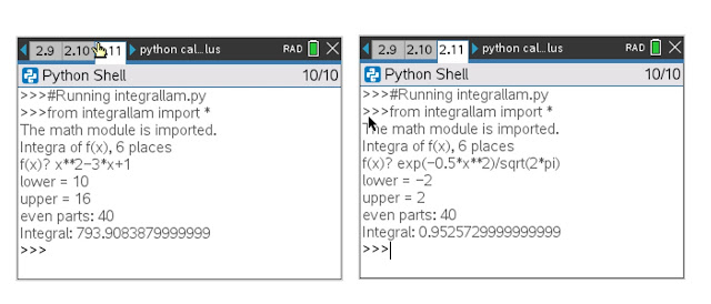
integrallam.py:  Numeric Integer


from math import *


print("The math module is imported.")

print("Integra of f(x), 6 places")

f=eval("lambda x:"+input("f(x)? "))


# input parameters

a=eval(input("lower = "))

b=eval(input("upper = "))

n=int(input("even parts: "))


# checksafe, add 1 if n is odd

if n/2-int(n/2)==0:

  n=n+1


# integral calculus

s=f(a)+f(b)

w=1

# 1 to n-1

for i in range(1,n):

  w=f(a+i*(b-a)/n)

  s+=(2*w) if (i/2-int(i/2)==0) else (4*w)

s*=(b-a)/(3*n)

print("Integral: "+str(round(s,6)))


All original content copyright, © 2011-2022.  Edward Shore.   Unauthorized use and/or unauthorized distribution for commercial purposes without express and written permission from the author is strictly prohibited.  This blog entry may be distributed for noncommercial purposes, provided that full credit is given to the author. 

Python - Lambda Week: Derivatives and Newton's Method

Python - Lambda Week: Derivatives and Newton's Method


Welcome to Python Week!  This we we're going to cover calculus and the keyword lambda.


Note:  All Python scripts presented this week were created using a TI-NSpire CX II CAS.   As of June 2022, the lambda keyword is available on all calculators (in the United States) that have Python.   If you are not sure, please check your calculator manual. 


Derivative


The Five Stencil Method is used.  Due to the approximate nature, results are rounded to 5 digits.


f'(x) ≈ (-f(x+2*h) + 8*f(x+h) - 8*f(x-h) + f(x-2*h)) / (12 * h)


h is set to 0.0001 to allow for a wide range of functions and to hopefully prevent float point overflows or underflows.  You can modify h or have the user input a value if you so wish.  


derivlam.py:  Derivative Using the Five Stencil Method


# Math Calculations

#================================

from math import *

#================================


print("The math module is imported.")

f=eval("lambda x:"+input("f(x)? "))


# input x0

x=eval(input("d/dx at x0: "))

h=.0001


# derivative, 5 stencil

d=(-f(x+2*h)+8*f(x+h)-8*f(x-h)+f(x-2*h))/(12*h)

print("round to 5 decimal points")

print("d/dx = "+str(round(d,5)))


Newton's Method


The next script finds the root of f(x) (solve f(x) = 0) with a guess.  


x_n+1 = x_n - f(x_n) / f'(x_n)


The derivative is calculated using the Five Stencil Method.   


I put a limit of 100 iterations because Newton's Method is not always perfect nor this script finds solutions in the complex plane, just the real numbers.  


newtonlam.py


# Math Calculations

#================================

from math import *

#================================

print("The math module is imported.")

print("Solve f(x)=0 to 6 places")

f=eval("lambda x:"+input("f(x)? "))


# input x0

x=eval(input("Guess? "))

h=.0001


w=1

n=1

while fabs(w)>10**(-7):

  d=(-f(x+2*h)+8*f(x+h)-8*f(x-h)+f(x-2*h))/(12*h)

  w=f(x)/d

  x-=w

  n+=1

  if n>100:

    print("iterations exceeded")

    break


if n<101:

  print("x = "+str(round(x,6)))

  print("iterations used: "+str(n))


All original content copyright, © 2011-2022.  Edward Shore.   Unauthorized use and/or unauthorized distribution for commercial purposes without express and written permission from the author is strictly prohibited.  This blog entry may be distributed for noncommercial purposes, provided that full credit is given to the author. 


TI-58/TI-59 Week: Numerical Derivative

TI-58/TI-59 Week:  Numerical Derivative


Introduction


The program estimates the numeric derivative:


d/dx f(x) = (f(x + h) - f(x)) / h


Registers used:

R01:  x

R02:  h

R03:  d/dx


Labels:

[ A ]:  store x

[ B ]:  store h

[ C ]:  calculate derivative


LBL E:  store f(x), assume x is in the display.  You can use registers R00 and R06 and above for registers.  Use Rad  ( [ 2nd ] [ - ] ) if f(x) contains trigonometric functions.  End each function with the steps =, INV SBR (RTN)


Function Listings


(step number, key code, key)


000 76 LBL

001 11 A

002 42 STO

003 01 01

004 92 INV SBR (RTN)


005 76 LBL

006 12 B

007 42 STO

008 02 02

009 92 INV SBR (RTN)


010 76 LBL

011 13 C

012 43 RCL

013 01 01

014 85 +

016 43 RCL

017 02 02

018 71 SBR

019 15 E

020 42 STO

021 03 03

022 43 RCL

023 01 01

024 71 SBR

025 15 E

026 94 +/-

027 85 +

028 43 RCL

029 03 03

030 95 =

031 55 ÷

032 43 RCL

033 02 02

034 95 =

035 42 STO

036 03 03

037 92 INV SBR (RTN)


038 76 LBL

039 15 E

...      .... ....

n-1 95 =

nnn 92 INV SBR (RTN)


Examples


f(x) = sin x;    Rad, sin


x = 0.5, h = 0.1, [ C ] returns 0.8521693479

x = 0.5, h = 1E-8, [ C ] returns 0.87755


f(x) = (1 + cos x)^1.5;   Rad, cos, +, 1, =, y^x, 1.5


x = 2, h = 0.01, [ C ] returns -1.035743295

x = 2, h = 1E-8, [ C ] returns -1.04206


f(x) = x * e^(x);   STO, 00, e^x * RCL, 00


x = 3, h = 0.01, [ C ] returns 80.84630054

x = 3, h = 1E-5, [ C ] returns 80.342648


Eddie


All original content copyright, © 2011-2022.  Edward Shore.   Unauthorized use and/or unauthorized distribution for commercial purposes without express and written permission from the author is strictly prohibited.  This blog entry may be distributed for noncommercial purposes, provided that full credit is given to the author. 


Calculus: Scaled Integration

Calculus:  Scaled Integration


Introduction


The take the integral:


∫( f(x) dx, A, B) 


The integral can be transformed to new limits C and D via linear transformation:


∫( f(x) dx, A, B) → ∫( g(y) dy, C, D)


Where the interval [ C, D ] has the smaller range than [ A, B ].


Set the transformation to:


y = m*x + β


C = m*A + β

D = m*B + β


Solving for m, β:


(C - D) = (A - B) * m

m = (C - D) / (A - B)


and


β = C - A * m = D - B * m


Solving y = m*x + β for x:


x = 1/m * (y - β)


Taking the derivative of both sides:


dx = 1/m  dy


The transformed integral:


∫( f(x) dx, A, B) → 1/m * ∫( f(1/m * (y - β)) dy, C, D)


Examples


Example 1:  


∫(x^2 - 5 dx, 10 ,16) but scale the integration interval to [1, 2].


A = 10, B = 16, C = 1, D = 2

m = (1 - 2)/(10 - 16) = 1/6,  1/m = 6

β = 1 - 10 * 1/6 = -2/3

x = 6 * (y + 2/3) = 6 * y + 4


Transformed Integral:

6 * ∫( (6*y + 4)^2 - 5 dy, 1, 2) = 1008


Example 2:


∫( e^x * ln(x + 2) dx, 0, 5) but scale the integration to [0, 1].


A = 0, B = 5, C = 0, D = 1

m = -1/-5 = 1/5,  1/m = 5

β = 0 - 0 * 1/5 = 0

x = 5 * y


Transformed Integral:

5 * ∫( e^(5 * y) * ln(5 * y + 2) dy, 0, 1) ≈ 262.8586594


Numerical integrals were calculated with the TI-36X Pro.  


When trying the Simpson's rule or Trapezoid rule, I find the smaller range does not really give better estimates.  But I am presenting the technique and if this helps in the future, great.  


Coming up:


July 11 - July 15, 2022:  TI-58 and TI-59 Week

Next Regular Blog:  July 23, 2022


Eddie  


All original content copyright, © 2011-2022.  Edward Shore.   Unauthorized use and/or unauthorized distribution for commercial purposes without express and written permission from the author is strictly prohibited.  This blog entry may be distributed for noncommercial purposes, provided that full credit is given to the author. 


Plus42: Integration in Solver

Plus42: Integration in Solver


The Plus42 adds an integral function to the solver engine.


Just a Reminder:  Get the Plus42 App


Author:  Thomas Okken


App: 

Android:  $9.99

iOS:  $9.99

PC/MacOS/Linux:  Free

Donations Accepted


Link:  https://thomasokken.com/plus42/


Plus42 ∫ Syntax


∫(EXPR:VAR:LLIM:ULIM[:ACC])


EXPR:  expression to be integrated


VAR:  variable to be integrated


LLIM: lower limit


ULIM:  upper limit


ACC:  accuracy factor, an optional argument.  If ACC is omitted, then Plus42 uses the highest accuracy factor.   


Let's take a look at some of the integrals that can be used.  In this blog, all results are rounded to four decimal places (FIX 4 is the default setting of Plus42)


Example 1:  Basic Integral


I = ∫(x^2 + 1 dx, x = 0, 3)


Solver syntax:

I=∫(X^2+1:X:1:6)


This integral calculates the numerical integral of x^2 + 1 from x = 1 to x = 6.   In calculation mode, pressing ( I ) twice would definitely get the result.  


Result:  I=76.6667


Example 2:  Variable Upper Limit


I = ∫(x^3/3 - 2 dx, x = 0, A),   A is the upper limit


Solver syntax:

I=∫(X^3÷3-2:X:0:A)


Upper limit known, find the integral:

A = 4;  result:  I = 13.3333


Integral known, find the upper limit:

I = 4;  result:  A = 3.3692 (it may take have time depending on the initial guess)


I like how the solver can find both the value of the integrals and solve for the limits of the integral.


Example 3:  Variable in the Integrand


I = ∫((x^2 * (x - B)) / (B^2 + x^2) dx, x = 0, 1),  B is a variable constant


Solver syntax:

I=∫((X^2×(X-B))÷(B^2+X^2):X:0:1)


B = 1; I = -0.0612

B = 3; I = -0.0784  (I set the initial guess of I = 0)


B can be solved for if you have a good guess and you are willing to wait for the solver to work.


I = -0.07; B = 3.6139


Full Precision:  3.613900797617638382718999085866498


Eddie 


All original content copyright, © 2011-2022.  Edward Shore.   Unauthorized use and/or unauthorized distribution for commercial purposes without express and written permission from the author is strictly prohibited.  This blog entry may be distributed for noncommercial purposes, provided that full credit is given to the author. 


Casio fx-4000P: Orthonormal 2D Vector Test

Casio fx-4000P:  Orthonormal 2D Vector Test


Introduction


A set of vectors form an orthonormal basis if the vectors are mutually perpendicular and are of unit length.  


Mutual perpendicular means the dot product of two different vectors in the space is 0:


v_i ∙ v_j = 0,  i ≠ j


Unit length means that the norm of each vector is 1:


|v_i| = 1


 For two 2D vectors [ A, B ] and [ C, D ], the two vectors form an orthonormal basis if:


A^2 + B^2 = 1

C^2 + D^2 = 1

A * D + B * C = 0


Casio fx-4000P Program:  Orthonormal 2D Vector Test

Bytes:  84 steps

(line returns are included for readability)


"A":

?→A:

"B":

?→B:

"C":

?→C:

"D":

?→D:

A²+B²≠1⇒Goto 0:

C²+D²≠1⇒Goto 0:

AD+BC≠0⇒Goto 0:

"YES" ⊿

Goto 1:

Lbl 0:

"NO" ⊿

Lbl 1


Examples


Example 1:

[1, 0], [0, 1]

A = 1, B = 0, C = 0, D = 1


"NO"   (1*1 - 0*0 = 1)


Example 2:

[1/√2, 1/√2], [1/√2, -1/√2]

A = 1/√2, B = 1/√2, C = 1/√2, D = -1/√2


"YES"


Source:


Rowland, Todd. "Orthonormal Basis." From MathWorld--A Wolfram Web Resource, created by Eric W. Weisstein. https://mathworld.wolfram.com/OrthonormalBasis.html

Last Accessed April 7, 2022


Eddie 


All original content copyright, © 2011-2022.  Edward Shore.   Unauthorized use and/or unauthorized distribution for commercial purposes without express and written permission from the author is strictly prohibited.  This blog entry may be distributed for noncommercial purposes, provided that full credit is given to the author. 


Backlink 9999 Traffic Super

Order Now...!!!!